Office hours: Mon, Wed, Fri 12:30−2:00, and after class, and by appointment.
Lecture: Mon, Wed, Fri 11:30−12:20 in Wells A-224
Assistant: Clara Mussin Phillips, mussinph@msu.edu
Recitation: Thu 10:20-11:40 in Berkey 219
MLC hours: Mon 12:30-1:40, Thu 12:30-4:00 in Wells C lobby.
- Last-minute study help:
- Office hours: Fri Dec 5, 12:30-2:00pm, Wells D-326
- Student vector parties: Sun Dec 5, 6:30-8:30pm & Tue Dec 10, 12:00-2:00pm, both in Engineering Bldg 1225
- Extra office hours: Tue Dec 10, 2:00-3:30pm, Wells D-326. (No office hours Mon.)
- WHW 11
due Wed 12/11: Final review problems.
(tex)
- Extra Review Material: Syllabus and extra problems below.
- Final Exam:
Wed Dec 11, 7:45-9:45am in our usual classroom Wells A-224.
Solving (not just looking at) problems is essential to learning: only look at the solution after a serious effort.
I will give 1 extra point to the first person reporting each significant typo or error on this page. Corrections and recent revisions are in red. Tentative future assignments are in gray.
- 8/28 Lect 1.
⊞
Vectors v,u ∈ R2, dot product
u•v, orthogonal decompostion v = p+q.
⊞ Solutions
- We write a vector v interchangeably as:
- two-point form v = AB, the arrow from point A to B; the same v could be drawn starting at any point in the plane;
- standard form v = (x,y) ∈ R2, giving the endpoint if v is drawn starting at (0,0).
- Operations sv, u ± v; basis vectors i = (1,0), j = (0,1), v = (x,y) = xi + yj
- Parametrized segment from a to b: a + t(b−a) = (1−t)a + tb for 0 ≤ t ≤ 1
- Dot product u•v = ±|u| |p| = |u| |v| cos(θuv), where p = perpendicular projection of v on u-line
- Length |v| = √(v•v), orthogonality u•v = 0, unit vector v⁄|v|
- Properties: commutative, bilinear, basis ⇒ formula:
u•v = (u1,u2) • (v1,v2) = u1v1 + u2v2 - Angle computation:
θuv = arccos u•v⁄|u||v| = arccos (u1v1+u2v2) ⁄√(u12+u22) √(v12+v22) - Orthogonal decomposition v = p + q with p||u , q⊥u ⇒ p = (v•u)⁄(u•u) u and q = v − p
HW 1: Start the Weekly Homework WHW 1 due 8/30 below.- Consider the triangle with vertices A = (1,2), B = (3,3), C = (2,0). Use dot products to show this is a right triangle, and verify the Pythagorean Theorem.
- Consider vectors v = (0, −10) and u = (3,2),
and let v = p + q be the orthogonal decomposition
where p is parallel to u
and q is orthogonal to u.
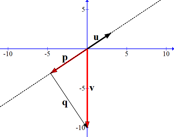
- Find the length |p| by computing the dot product u • v, then recalling our original definition u • v = ±|u| |p|, so that |p| = u•v⁄|u| .
- Find p and q by finding the scalar t such that
p = tu is perpendicular to q = v − tu.
Hint: Solve for t in the equationtu • (v − tu) = 0. Deduce the formulas for p, q in the notes above. Apply this formula to the specific u, v. - If u points along an inclined plane, and v represents the acceleration for a free-falling object (about 10 m/sec2), then what is the acceleration of an object sliding without friction along the plane? What is the gravitational force of a unit-mass object against the plane?
- Show that for u = (u1, u2), the vector u⊥ = (−u2, u1) is perpendicular to u. Since the above q is the projection of v on u⊥, we should have q = (v•u⊥)⁄(u⊥•u⊥) u⊥. Verify this for the specific u, v above.
- Given a triangle whose vertices are (the endpoints of)
u, v, w,
the centroid or center of gravity is:
c = 1⁄3(u + v + w), the point whose x-coordinates are the average of the x-coordinates of the vertices, and same for y-coordinates.
A median of the triangle is the line segment from a vertex to the midpoint of the opposite side.
Using vector algebra, prove that the three medians all intersect at the centroid, which is 2⁄3 of the way along each median.- Write each median as a parametrized line segment.
- Show that the point 2⁄3 of the way along each median is indeed the centroid.
- [MT] Ch 1.2 Exercise 27, 29, 31, 33, 37, 39. Ch 1 Review Ex 19, 39.
1. Consider the vectors a = OA, b = OB, c = OC, and let α be the angle at A. Then:
cos(α) = (b−a)•(c−a)⁄|b−a| |c−a| = (2,1)•(1,−2)⁄√5√5 = 0. Thus α = arccos(0) = π⁄2, a right angle, and similarly for the other two angles. The Pythagorean Theorem says |b−a|2 + |c−a|2 = |c−b|2, i.e. (√5)2 + (√5)2 = (√10)2.2a. We compute: |p| = |u•v|⁄|u| = |(3,2)•(0,−10)|⁄|(3,2)| = 20⁄√13.
2b. Given u, v, we solve for the scalar t in the equation tu • (v−tu) = 0, namely tu•v − t2u•u = 0, and t = (u•v)⁄(u•u). This gives the familiar projection formula p = (u•v)⁄(u•u) u = −(60⁄13,40⁄13) and q = v − p = (60⁄13,−90⁄13).
2c. Here p is the component of acceleration along the plane u, so the acceleration is |p| = 20⁄√13 ≈ 5.5 m/sec2, about half the acceleration of free-fall. The force on the surface is mass times the perpendicular acceleration, so a 1 kg object (pressing about |v| = 10 Newtons on a flat surface) would exert a force of |q| = 30⁄√13 ≈ 8.3 N.
4. Odd-numbered exercises in [MT] have answers in the back, p. 494.
- We write a vector v interchangeably as:
- 8/29 Recitation 1. Geometric theorems through vector algebra, Weekly Home Work 1.
- 8/30 Lect 2.
⊞
Linear fun ℓ, directional distance ℓ(v) = m•v
⊞ Solutions
- Linearity property: ℓ(u+v) = ℓ(u) + ℓ(v) , ℓ(sv) = s ℓ(v).
affine function: f(v) = ℓ(v) + b
ℓ : R → R, ℓ(x) = mx , f(x) = mx + b - ℓ : R2 → R,
ℓ(v) = m•v
= scaled distance function in m direction
true distance = m⁄|m| • v , where m⁄|m| is a unit vector (length 1)
affine function f(v) = m•v + b
countour map shows plane R2 with countour lines defined by ℓ(x,y) = const
- Recall from HW 1 that the orthogonal decomposition of a vector v with respect to direction u is:
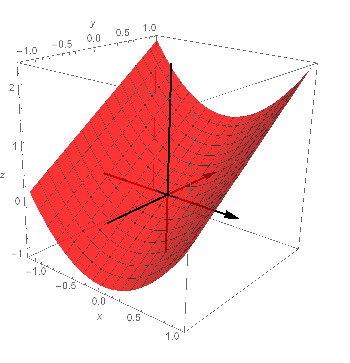
v = p + q where p = (v•u)⁄(u•u) u, q = v − p. Apply this to find the orthogonal decomposition of a general v = (x,y) with respect to direction u = (1,1). - Define the function ℓ(x,y) to be the distance of the point (x,y) above the line y = x; that is, the distance of (x,y) from the closest point the line. Points above the line (with x < y) have positive ℓ(x,y), while points below (with x < y) have negative ℓ(x,y).
Problem: Write ℓ as a linear function ℓ(v) = m•v = m1x + m2y, for a particular direction m = (m1,m2).
Hint: The distance of v above the line is the length of the projection q from #1. - Picture the above function ℓ(x,y).
- Draw the contour map showing sample lines ℓ(x,y) = −1, ℓ(x,y) = 0, ℓ(x,y) = 1, etc.
- Use Wolfram Alpha
to draw the 3D graph: plot z = ℓ(x,y), where you write the explicit formula for ℓ(x,y).
Hint: Write a square root √a as a^(1/2).
1,2. The projection of the vector v = (x,y) orthogonal to direction u = (1,1) is:q = (x,y) − (x+y)⁄2 (1,1) = (x−y)⁄2 (1,−1) . This has signed length:ℓ(x,y) = ±(x−y)⁄√2 = ±(1⁄√2,−1⁄√2) • (x,y). Since we defined ℓ(−1,1) > 0 and ℓ(1,−1) < 0, we see that ± in the above formula should be −, so that:ℓ(x,y) = (−x+y)⁄√2 = (−1⁄√2,1⁄√2) • (x,y). 3. See Wolfram Alpha for both plots.
- Linearity property: ℓ(u+v) = ℓ(u) + ℓ(v) , ℓ(sv) = s ℓ(v).
- 9/2 Labor Day, no class
- 9/4 Lect 3. Linear mappings L : R2 → R2. Notes & WHW 2.
- 9/5 Recitation 2. Linear mappings, matrix multiplication, WHW 2.
- 9/6 Lect 4.
⊞
Matrix notation [L] for linear transformation L
Solutions
- A matrix of size (m×n) is a table of numbers with m rows and n columns.
- ℓ : R2 → R , ℓ(v) = m•v = ax + by for m = (a,b), v = (x,y)
Matrix notation: (1×2) • (2×1) = (1×1), dot row with column[ℓ] • [v] = a b • x y = ax + by = ℓ(v) - L : R2 → R2 defined by
L(i) = (a,b), L(j) = (c,d),
L(v) = L(x,y) = x(a,b) + y(c,d) = (ax+cy, bx+dy) Matrix notation: (2×2) • (2×1) = (2×1), dot rows of [L] with column [v]
= ( (a,c)•(x,y) , (b,d)•(x,y) )
That is, [L(v)] = M • [v] , where M = [L] = "matrix of slopes"[L] • [v] = a b c d • x y = a c b d • x y = (a,c)•(x,y) (b,d)•(x,y) = [L(v)] - Composition of linear transformations: L1(L2(v)) = L3(v), with linear L3 : R2 → R2
[L1] = a b c d = a c b d , [L2] = e f g h , [L3] = ??
Answer: to get [L3], dot rows of [L1] with columns of [L2].[L3] = [ L1(L2(i)) | L1(L2(j)) ] = [ [L1]•[L2(i)] | [L1]•[L2(j)] ] = (a,c)•(e,f) (a,c)•(g,h) (b,d)•(e,f) (b,d)•(g,h) - Matrix multiplication rule: (m×k) • (k×n) = (m×n)
Product matrix ith row, jth column is equal to: ith row of first dotted with jth column of second.− r1 − ⋮ − rm − • | c1 | . . . | cn | = r1• c1 . . . r1• cn ⋮ ⋮ rm• c1 . . . rm• cn - Chain Rule for Linear Transformations: If we define the composition L3(v) = L1(L2(v)), then we have the matrix equation [L3] = [L1] • [L2].
- We can write dot product in terms of matrix product
using the matrix-transpose: if [v] denotes a
n×1 column vector, we write [v]T
to mean the 1×n row vector. Then:
v•w = [v]T [w].
HW 4:- For a unit vector u = (u1, u2) = (cos(θ), sin(θ)) with |u| = 1, let Proju(v) : R2 → R2 be the orthogonal projection of v onto direction u.
- Find the matrix of Proju.
- Use matrix multiplication to find the matrix of the composition Proju ∘ Proju, and explain the result geometrically.
- Find Proju ∘ Projw for w orthogonal to u, and again explain the result geometrically.
- Consider the two linear mappings ℓ1 : R2 → R , ℓ1(v) = m•v , and ℓ2 : R → R2 , ℓ2(t) = ta. Of the four possible compositions, ℓ1∘ℓ1 , ℓ1∘ℓ2 , ℓ2∘ℓ1 , ℓ2∘ℓ2 , which ones are defined (make sense)? For each composition which does make sense, adapt the Chain Rule (matrix multiplication) to compute its matrix, and describe the mapping geometrically.
- Assume the fact that a composition of rotations is a rotation: Rotα ∘ Rotβ = Rotα+β. Use the Chain Rule to translate this into an equality of matrices, and prove the Angle Addition Formulas for sin(θ) and cos(θ). This is the "real" reason for these formulas.
- [MT] Ch 1.5 Ex 17: Is multiplication of 2×2 matrices always commutative, A•B = B•A ?
- 9/9 Lect 5.
⊞
Parametrized curve c(t), scalar-valued fun f(x,y), graph, contour plot
⊞ Solutions
- Parametrized curve c : R → R2 , c(t) = (x(t), y(t))
- Example: cycloid c(t) = (0,1) + (t,0) − (sin(t),cos(t))
- Parametric curve plotter, 3D-graph plotter
- Scalar-valued f : R2 → R.
Pictures: draw graph z = f(x,y), contour map of level curves f(x,y) = c
Examples:- Linear f(v) = ℓ(v) = m•v
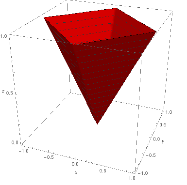
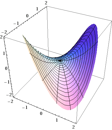
- Cone f(v) = |v| ,
paraboloid f(v) = |v|2 = x2+y2 ,
surface of revolution f(v) = g(|v|) for one-var g(r) - Trough f(x,y) = x2, vertical slices
- Saddle surface f(x,y) = x2−y2, vertical and horiz slices
HW 5: Look at the new WHW 3 due 9/13 below.- Consider the curve C in the plane defined by |x| + |y| = 1. Describe this in three ways.
- Write C as the combined graphs of two functions y = ±f(x).
- Parametrize C by c(t) = (x(t),y(t)). Define c(t) piecewise: for 0 ≤ t ≤ 1, let c(t) parametrize the segment from (x,y) = (1,0) to (0,1), and similarly for 1 ≤ t ≤ 2, etc.
- Write C as a level curve of a two-variable function f(x,y) = c. Draw the graph z = f(x,y), indicating the level curves.
- Picture each of the following functions f : R2 → R by drawing:
- its contour map, a set of level curves f(x,y) = c for c = . . . ,−1, 0, 1, . . .
- its graph z = f(x,y), by stacking level curves and/or assembling vertical slice curves (ribs)
- f(x,y) = x + 3y
- f(x,y) = x2 + y
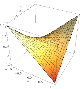
- f(x,y) = xy
- f(x,y) = x3 − 3x − y2
- Extra Credit: For each curve below, possibly described in polar coordinates, find a parametric form c(t) = (x(t), y(t)), and
plot it with Wolfram Alpha. Prove the claimed properties.
- Lemniscate of Bernoulli: r = a √(cos(2 theta)).
- This is a hyperbola inverted by the mapping T(v) = v⁄|v|2 , which takes the reciprocal of the radius. That is, T(hyperbola) = lemniscate.
- It has two focus points F, F' such that every point P of the curve has the product of distances to the foci equal to the square of the distance between the foci: (PF) (PF') = (FF')2.
- It is the curve we get if we take vertical slice a torus (donut) by a plane tangent to the inner ring.
- Lissajous curves c(t) = (sin(at+c), sin(bt)) for various constants a,b.
- Rose petal curves r = cos(kθ), 2k petals for k even, k petals for k odd
- Cardioid epicycloid r = 2a(1+cos(θ)) or off-center r = 4a cos2(½θ)
- This is the inversion by T of a parabola whose infinite part is toward the positive x-axis.
- This is the curve traced by a point on the edge of a circle rolling around a cirle of the same radius.
- Lemniscate of Bernoulli: r = a √(cos(2 theta)).
1a. Two graphs y = 1−|x| and y = −(1−|x|) for −1 ≤ x ≤ 1.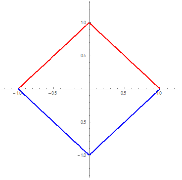
1b. Four parametrized segments along 0 ≤ t ≤ 4:
- c(t) = (1,0) + (−1,1)t for 0 ≤ t ≤ 1
- c(t) = (0,1) + (−1,−1)(t−1) for 1 ≤ t ≤ 2
- c(t) = (−1,0) + (1,−1)(t−2) for 2 ≤ t ≤ 3
- c(t) = (0,−1) + (−1,1)(t−3) for 3 ≤ t ≤ 4
1c. For f(x,y) = |x| + |y|, our curve is the level curve f(x,y) = 1. Graph:
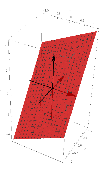
2a. f(x,y) = x + 3y. Level curves: f(x,y) = c , y = −⅓x + k parallel lines. Ribs: z = f(x,c) = x + k , z = f(c,y) = 3y + k lines.
2b. f(x,y) = x2 + y . Level curves: f(x,y) = c , y = −x2 + k parabolas. Ribs: z = f(x,c) = x2 + k upward parabolas , z = f(c,y) = k + y lines.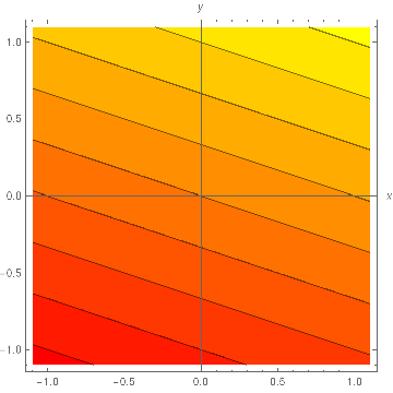
2c. f(x,y) = xy . Level curves: f(x,y) = c , y = c⁄x hyperbolas. Ribs: z = f(x,c) = cx , z = f(c,y) = cy steeper & steeper lines, z = f(x,x) = x2 upward parabola, z = f(x,−x) = −x2 downward parabola.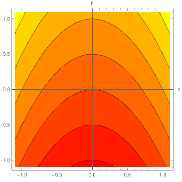
2d. f(x,y) = x3 − 3x − y2 . Level curves: f(x,y) = c , y = √(c − x3 + 3x) ?? Ribs: z = f(x,c) = x3 − 3x − k cubic with hill & valley, z = f(c,y) = − y2 + k downward parabola.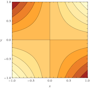
- 9/11 Lect 6.
⊞
Lin approximations DF: c'(a), ∂f⁄∂x(a,b),
∇f(a,b).
⊞ Solutions
-
For f : R → R, deriv f '(a) is slope of best (affine) linear approx:
f(x) ≈ f(a) + f '(a)(x−a) for x ≈ a, or f(a+h) ≈ f(a) + f '(a) h -
Deriv of c(t) at t = a: best linear approx for t ≈ a,
c(t) ≈ c(a) + c'(a) (t−a) = tangent line; or c(a+h) ≈ c(a) + c'(a) h
Find c'(a) = ?? From calculus, approximate each component:
(x(a+h), y(a+h)) ≈ (x(a) + x'(a) h , y(a) + y'(a) h) = c(a) + (x'(a),y'(a)) h.
Thus: c'(a) = (x'(a), y'(a)) -
Deriv of f : R2 → R is best linear approx
for v ≈ a = (a,b),
f(v) ≈ f(a) + ∇f(a)•(v−a) = tangent plane, or f(a+h) ≈ f(a) + ∇f(a)•h
Gradient vector ∇f(a) = (d1, d2) = ??
f(a+h, b) ≈ f(a,b) + (d1,d2)•(h,0) = f(a,b) + d1h
Thus: d1 = d⁄dxf(x,b)|x=a = ∂f⁄∂x(a,b); similarly d2 = d⁄dyf(a,y)|y=b = ∂f⁄∂y(a,b) -
Tangent plane approx for (x,y) near (a,b):
f(x,y) ≈ f(a,b) + ∂f⁄∂x(a,b) (x−a) + ∂f⁄∂y(a,b) (y−b)
Partial derivative ∂f⁄∂x(a,b) is slope in x-direction -
Gradient is vector of partial derivatives:
∇f(a) =
(∂f⁄∂x(a), ∂f⁄∂y(a))
Gradient vector field: ∇f(v) gives an arrow at each v = (x,y).
Draw gradient field for examples from previous Lect.
Vector field plotter
Fact: ∇f(a) is uphill direction, length = uphill slope
HW: Look at WHW 3 due 1/27 below.- Consider the curve c(t) = (t2, t3) for t ∈ (−∞, ∞).
- Draw the curve by hand-plotting points for some sample t-values, then check this against a computer plot.
- Solve for t as a function of x, and use this to write y = f(x), possibly needing more than one graph. Sketch this graph, and compare the result with part (a).
- Find the tangent vector c'(t) at t = 1. Zoom in on your plot of c(t) near c(1) and verify that the curve looks indistinguishable from the parametrized line c(1) + c'(1)(t−1). (Here c'(1) is the velocity vector of a particle moving along c(t), at time t = 1; the length |c'(1)| is its speed.)
- The tangent vector at t = 0 is zero. How to describe the corresponding motion of a particle along c(t)?
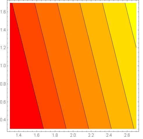
- Consider the function f : R2 → R given by
f(x,y) = x2 + y, near the point (x,y) = (2,1).
- Compute the linear approximation f(x,y) ≈ f(2,1) + ∇f(2,1)•(x−2,y−1) for (x,y) ≈ (2,1).
- Zoom in on the contour map of f(x,y) near (x,y) = (2,1). Compare it with contour map of the approximation g(x,y) = f(2,1) + ∇f(2,1)•(x−2,y−1). If you zoom enough, the two should look the same: this is the defining property of the derivative ∇f(2,1).
- Draw the gradient vector ∇f(2,1) onto the contour map of f, starting at (2,1). Note that it is perpendicular to the level curve through (2,1), and points uphill, in the direction of maximum increase of f.
- For each function f(x,y) = x+3y, x2+y, from the previous HW Ex #2a,b, compute the derivative (gradient vector) ∇f(x,y) = (∂f⁄∂x(x,y), ∂f⁄∂y(x,y)). At grid points (x,y), draw ∇f(x,y) as an arrow starting at (x,y): this is the gradient vector field, another way of picturing f. (Use the computer if it's too complicated.) Compare the gradient field with the contour map of the function in the previous HW solutions, and verify that the gradient vectors are perpendicular to the level curves f(x,y) = c. Also verify: closer level curves ⇔ steeper 3D-graph slope ⇔ longer gradient vector.
- (p 124 #24) Consider the exponential spiral given
by: c(t) = (et cos(t), et sin(t)).
Show that the angle between the radial vector c(t)
and the velocity vector c'(t) is constant for all t.
This is why a moth flies in a spiral path around a flame: it is trying to navigate in a straight line by keeping the moon or a star at a constant angle in its field of vision.
1a. c(t) = (t2, t3)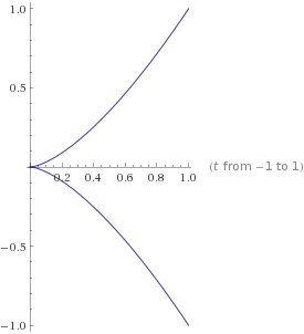
1b. Eliminating t from the system of equations {x = t2 , y = t3} gives t = ±√x, and y = ±x3/2 (two graphs). The function x3/2 rises faster than y = x, but not as fast as y = x2.
1c. The derivative is: c'(t) = (2t, 3t2), so c'(1) = (2,3). The linear approximation (red tangent line) is:
ℓ(t) = c(1) + c'(1)(t−1) = (1,1) + (2,3)(t−1) = (2t−1, 3t−2), which is very close to the original curve (black) even in a window of width 1.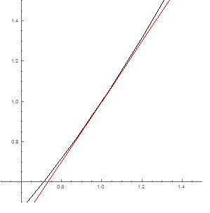
1d. c'(a) = 0 means zero velocity at time t = a. Here, the particle traveling along the curve slows down as it approaches time t = 0, stops, then gradually starts again in the opposite direction. No matter how it is represented, the curve has no well-defined tangent line at (x,y) = (0,0).
2a. The function f(x,y) = x2 + y has ∇f(x,y) = (2x,1), with ∇f(2,1) = (4,1). The linear approximation for (x,y) ≈ (2,1) is:
ℓ(x,y) = f(2,1) + ∇f(2,1)•(x−2,y−1) = 5 + (4,1)•(x−2,y−1) = 4x + y − 1. 2b. Comparing the plots of f(x,y) and the linear approximation ℓ(x,y) zoomed in near (2,1) shows they are very close:
2c. The gradient vector ∇f(2,1) = (4,1) is scaled down to fit in the picture above. Notice that it is perpendicular to the level curve f(x,y) = 5 through (2,1), and points toward the direction of fastest increase of f(x,y), shown by lighter colors in the contour map. To explain why, note that the linear approximation f(x,y) ≈ ℓ(x,y) = 5 + (4,1)•(x−2,y−1) measures the "height" of the vector from (2,1) to (x,y), considering direction (4,1) as "up": this "height" increases fastest exactly in the direction (4,1).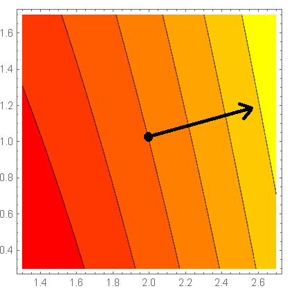
3a. f(x,y) = x + 3y , ∇f(x,y) = (1,3). That is, we draw the same vector (1,3) at each point (x,y), scaled down to fit the picture:
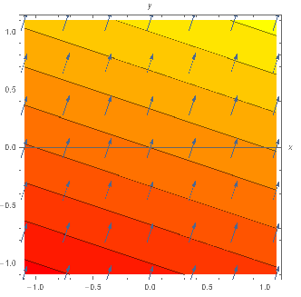
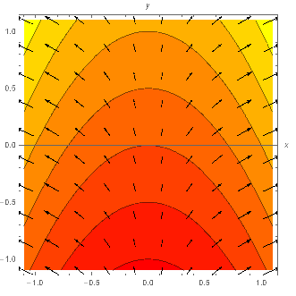
3b. f(x,y) = x2 + y , ∇f(x,y) = (2x,1). At a grid point (x,y), we draw an arrow (scaled) with vertical component 1, and horizontal component 2x: pointing to the right for x > 0, up for x = 0, and left for x < 0. Notice the vectors get longer near the sides, as the level curves get closer and the graph gets steeper.
4. The curve c(t) = et (cos(t), sin(t)) has derivative (velocity vector, tangent vector) given by the product rule:
c'(t) = (et)' (cos(t), sin(t)) + et (cos(t), sin(t))'
= et (cos(t)−sin(t), sin(t)+cos(t)),and we have |c(t)| = et, and |c'(t)| = et √2. A constant angle between c(t) and c'(t) would mean a constant dot product between the corresponding unit vectors:
cos θcc' = c⁄|c| • c'⁄|c'|
= (cos(t), sin(t)) • 1⁄√2 (cos(t)−sin(t), sin(t)+cos(t)) = 1⁄√2 .Thus θcc' = ±π⁄4 .
The moth would go inward along the path c(−t) with tangent −c'(−t), and it would see the flame at the origin in the direction −c(−t), which would give the same constant angle π⁄4 .
Last day for course changes in Math Office, Wells C-212 -
For f : R → R, deriv f '(a) is slope of best (affine) linear approx:
- 9/12 Recitation 3. Graph landscape, WHW 3
- 9/13 Lect 7.
⊞
Directional deriv ∂f⁄∂v = ∇f•v.
Critical pts ∇f = (0,0), max/min probs
⊞ Solutions
- Draw gradient vector field ∇f(x,y) = (∂f⁄∂x(x,y), ∂f⁄∂y(x,y))
examples:
linear ax+by, paraboloid x2+y2, cone √(x2+y2).
Arrow at c = (a,b) represents linear approximation f(x,y) ≈ f(a,b) + m1(x−a) + m2(y−b)
for slopes (m1, m2) = ∇f(a,b), provided (x,y) is close to (a,b)
Analogy to 1-dim derivative vector field (& graph, level marks) - Directional deriv ∂f⁄∂v(c)
= limh→0 (f(c+vh)−f(c))/h
= slope of graph above line ℓ(t) = c+vt if unit vector |v| = 1
Lin approx f(c+vh) ≅ f(c) + ∇f(a)•vh ⇒ ∂f⁄∂v(c) = ∇f(c)•v - Max slope of graph =
max|v|=1 ∇f(c)•v
= maxθ |∇f(c)| cos(θ)
= |∇f(c)| = gradient length, when θ = 0, v = ∇f(c)⁄|∇f(c)| = gradient direction
Lesson: v = ∇f(a) is direction of fastest increase of f(v) from v = a
|∇f(a)| is maximum slope - Critical point: (a,b) where ∇f(a,b) = (0,0):
all dir derivs are zero, flat point of graph z = f(x,y)
also ∇f(a,b) = undefined, non-differentiable points
Types: max, min, saddle, ridge (graph & contour pictures) - To find max/min of f(x,y), candidates are critical points and boundary points
- Max/min example: A box of size (x,y,z) with fixed volume xyz = 1.
Minimize surface area: 4 sides & bottom, no top. Ans: x = y = ½z, half as tall as wide. - Max/min example: Closest approach between y = x2 and y = x−1.
- Parametrize (t, t2), (s, s−1), square dist fun D(s,t) = (t−s)2 + (t2−(s−1))2 = min
- Inspect contour map to find crit pt
- Solve
∂D⁄∂t = 0, ∂D⁄∂s = 0, add eqns
⇒ (t,s) =
(1⁄2 ,7⁄8)
Boundary t,s → ∞ makes D → ∞ = max - Gradient flow method to approximate min pt
Guess point co, follow ∇f(co) to better (lower) point c1 = c1 + ε ∇f(co) for fixed ε
- Consider the function f(x,y) = xy.
- Sketch the graph z = xy. Hint: Draw the vertical slices above the radial lines y=0, x=y, x=0, x=−y. The result should be familiar.
- Sketch the contour map of level curves xy = c. Hint: What curve is y = c/x?
- Sketch the gradient vector field ∇f(v). That is, compute the gradient ∇f(x,y) = (∂f⁄∂x(x,y), ∂f⁄∂y(x,y)), and at each grid point (x,y) = (a,b) draw the arrow ∇f(a,b).
- Explain why the critical point looks the way it does in the three pictures.
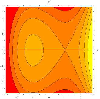
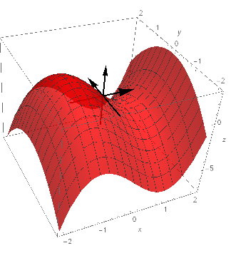
- For the function f(x,y) = x4 − 2x2 − 3(2x+1)y2,
have a computer draw its graph, contour map and gradient vector field.
Locate the critical points by
solving ∇f(x,y) = (0,0),
and verify the answers visually on your gradient plot.
Visually classify each critical point as:
- a local maximum (hill), where the gradient arrows all point in
- local minimum (bowl), where the arrows point out
- saddle point, where the arrows point in along one direction, out along another direction.
- ridge or ditch, where the vectors vanish along a ridgeline curve, with the surrounding vectors pointing toward (or away from) the ridgeline
Another example: f = 8x^2 - x^4 - 3y^2: max at (-2,0), (2,0), saddle at (0,0). Note f(x,y) = g(x) + h(y) with g'(x) = 4x(2-x)(2+x). Or: x3 − 3x − 3y2 - Max/min: Consider a rectangular bin having a bottom but no top, and three sides with the fourth side open. Assuming it has volume 1, find the
length, width and height which will minimize
the total surface area of the three sides and bottom.
Hint: Write the surface area as s(x,y), a function of the length x and width y (with the height z determined by volume = 1). Then the unique critical point, where ∇s(x,y) = (0,0), is the minimum point of s(x,y).
1a,b,c. f(x,y) = xy , ∇f(x,y) = (y,x).

2. f(x,y) = x4 − 2x2 − 3(2x+1)y2:
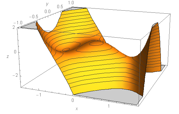
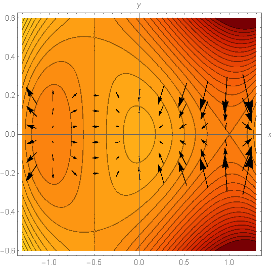
- (x,y) = (−1,0), a local min for f(x,y), a bowl in the graph, a darkening bullseye in the countour map, and an outflow point for the gradient vectors
- (x,y) = (0,0), a local max for f(x,y), a hill on the graph, a lightening bullseye in the contour map, and an inflow point for the gradient vectors
- (x,y) = (1,0), a pause point for f(x,y), a saddle point on the graph, an X on the countour map, with gradient vectors flowing in along the vertical direction and flowing out along the horizontal direction
- (x,y) = (−1⁄2, ±1⁄2), two more saddle points.
3. Letting x,y,z be the side-lengths of the rectangular bin, the volume is xyz = 1, and the surface area of the four sides is s = xy + yz + 2xz. Eliminating the variable z = 1⁄xy, we get the function
s(x,y) = xy + 1⁄x + 2⁄y for x,y > 0. The gradient field is: ∇s(x,y) = (y − 1⁄x2 , x − 2⁄y2):

The only critical point, where ∇s(x,y) = (y − 1⁄x2, x − 2⁄y2) = (0,0), is (x,y) = (2−1/3, 22/3) ≈ (0.8, 1.6). The vector field plot shows this is a local minimum, since the uphill vectors all point outward from this point. For completeness, we should also consider the critical points where ∇s is undefined, namely the boundary points where x = 0 or y = 0; but these are clearly vertical asymptotes where s(x,y) tends to infinity.
Thus, our final answer is: (x,y,z) = (2−1/3, 22/3, 2−1/3).
- Draw gradient vector field ∇f(x,y) = (∂f⁄∂x(x,y), ∂f⁄∂y(x,y))
examples:
- 9/16 Lect 8.
⊞
Anti-derivative via integral: f(b) − f(a) = ∫ab f '(x) dx
- Integral of f(x) over interval t ∈ [0,a]
Sample points 0 = t0 < t1 < ··· < tn = a, increments Δti = ti+1−ti
∫a0 g(t) dt = limn→∞ ∑ n=0 n−1 g(ti) Δti , limit of Riemann sums -
Ex: g(t) = sin(t), t ∈ [0,3⁄2]
sample points 0 < 0.5 < 1.0 < 1.5 , Δti = 0.5
∫01.5 sin(t) dt ≈ sin(0)(0.5) + sin(0.5)(0.5) + sin(1)(0.5) ≈ 0.66
More accuracy: extra sample points near start, where g(t) steeper
0 < 0.1 < 0.3 < 0.5 < 1.0 < 1.5
∫10 2t dt ≈ sin(0)(0.1) + sin(0.1)(0.2) + sin(0.3)(0.2)
+ sin(0.5)(0.5) + sin(1.0)(0.5) ≈ 0.74 - Fundamental Theorem:
Integral of rate of change is total change
∫0a f '(t) dt = f(a) − f(0).
Ex: Anti-derivative sin(t) = (−cos(t))', so:
∫01.5 sin(t) dt = (−cos(1.5)) − (−cos(0)) ≈ 0.93
Argument: linear approx for t ≈ ti , f(t) ≈ f(ti) + f '(ti)(t−ti),
so f-increment f(ti+1) − f(ti) ≈ f '(ti)(ti+1−ti) = f '(ti)Δti
∫0a f '(t) dt ≈ ∑ i=0 n−1 f '(ti) Δti ≈ ∑ i=0 n−1 (f(ti+1)−f(ti))
= f(tn) − f(t0) = f(a) − f(0)
Sum of f-increments equals total change in f
- Find the points on the curves y = x2 and y = x−1 which are closest to each other.
- Let f(s,t) be the square of the distance between points (s,s2) and (t,t−1). Compute f(s,t) and set up the optimization equations ∇f(s,t) = (0,0).
- Approximate the (unique) minimum point (s,t) using the Gradient Flow technique. That is, start with a reasonable guess po = (so, to), and improve this guess by moving straight downhill: p1 = po − ε ∇f(po). Now iterate to get a sequence of approximations po, p1, p2, . . . , continuing until the sequence stabilizes up to a desired accuracy. (Here ε is a constant such as ε = 1 or 0.5, which can be adjusted to get faster convergence.) Ans: Spreadsheet.
- Find the exact closest approach points (the minimum-distance points on the two curves). Hint: The shortest line segment between the two curves is perpendicular to them both. Thus, find the point where the parabola has slope 1, so that the perpendicular line has slope −1 and is also perpendicular to the line. Ans: (s,t) = (1⁄2, 7⁄8).
- Approximate the 1-variable integral
I = ∫10 e−t2 dt.
Note: This anti-derivative is not given by any formula, so only numerical methods work. Wolfram gives I ≈ 0.747, as well as an answer in terms of the Gaussian error function erf(t), but this is just defined in terms of the original integral. There is no way around approximation methods here.- Compute the Riemann sum by hand for n = 2 sample points, the left endpoint of each interval [ti, ti+1].
- Repeat part (a) for n = 10. (Use a spreadsheet.)
- Repeat part (a) for n = 2 with better sample points, the midpoints ti = ½(ti+ti+1). How much did this improve the accuracy from part (a)?
- Integral of f(x) over interval t ∈ [0,a]
- 9/18 Lect 9.
⊞
Reverse gradient via line integral: f(c(1)) − f(c(0)) = ∫c ∇f(c)•dc
⊞ Solutions
- Given vector field F(x,y) = ∇f(x,y),
define line integral to recover f(a,b).
Reverse the above argument.
Take curve c(t) with start c(0) = (0,0), end c(1) = (a,b).
Subdivide curve: 0 = t0 < t1 < . . . < tn = 1, points ci = c(ti)
Lin approx for v ≈ ci , f(v) ≈ f(ci) + ∇f(ci)•(v−ci)
so f-increment f(ci+1) − f(ci) ≈ ∇f(ci)•(ci+1−ci) = ∇f(ci)•Δci
Total change in f equals sum of f-increments:
f(a,b) − f(0,0) ≈ ∑ i=0 n−1 (f(ci+1)−f(ci)) = ∑ i=0 n−1 ∇f(ci)•Δci
Last expression approximates a new kind of integral: ∮c ∇f(c)•dc - Line integral of F(x,y) over curve
c(t) is defined as:
∮c F(c)•dc = limn→∞ ∑ i=0 n−1 F(ci)•Δci
for sample points c0 < ··· < cn on c(t), Δci = ci+1 − ci - Gradient Theorem: For any curve c(t) from (0,0) to (a,b):
∮c ∇f(c)•dc = f(a,b) − f(0,0).
We defined the line integral to make this true. - Ex: Field F(x,y) = ∇f(x,y) = (1, 6y),
integrated along c(t) = (t,t2) from (0,0) to (2,4)
sample points c0 = (0,0), c1 = (1,1), c2 = (2,4)
f(2,4)−f(0,0) = ∮c F(c)•dc ≈ F(0,0)•(c1−c0) + F(1,1)•(c2−c1)
= (1,0)•(1,1) + (1,6)•(1,3) = 20.
Guess anti-derivative: f(x,y) = x+3y2, ∇f(x,y) = (1,6y)
exact f(2,4)−f(0,0) = 50, approx 50 ≈ 20 stinks -
Improve approx: more sample points, or better:
sample midpoints ci = ½(ci+ci+1), keep previous Δci
Re-doing ex: c0 = (0.5, 0.5), c1 = (1.5, 2.5)
∮c F(c)•dc ≈ F(0.5, 0.5)•(c1−c0) + F(1.5, 2.5)•(c2−c1)
= (1,3)•(1,1) + (1,15)•(1,3) = 50, exact within error tolerance. - Reduce line integrals to ordinary integrals:
Sample points c(ti), c-increment Δci = c(ti+1)−c(ti+1) ≈ c'(ti) Δti, so:
∮c F(c)•dc ≈ ∑ i=0 n−1 F(ci)•Δci ≈ ∑ i=0 n−1 F(c(ti))•c'(ti) Δti ≈ ∫10 F(c(t))•c'(t) dt -
For F(x,y) = (p(x,y), q(x,y)) and a curve c(t) = (x(t),y(t)) for 0 ≤ t ≤ 1,
we can evaluate the line integral in terms of an ordinary one-variable integral:∮c F(c)•dc = ∫10 ( p(x(t),y(t)), q(x(t),y(t) ) • (x'(t),y'(t)) dt
= ∫10 p(x(t),y(t)) x'(t) + q(x(t),y(t)) y'(t) dt . - Ex: F(x,y) = (1,6y) for straight-line path to (2,4), and to (a,b)
Potential function f(a,b) = a + 3b2 + const -
Ex: F(x,y) = (−y,x) to (1,1) by straight line & by horiz/vert lines: different result
Inconsistency means F non-conservative, no potential function possible - Physical meaning: Work = force × distance
At time t, component of force along curve is F(c(t)) • c'(t)⁄|c'(t)|
Over time increment dt, distance = |c'(t)| dt
Work done by F in pulling along c is: ∫10 F(c(t)) • c'(t)⁄|c'(t)| |c'(t)| dt = ∮c F(c) • dc
Work done by F = − work needed to move against F
In physics, potential energy function φ(x,y) has ∇φ = −F
HW: Work on WHW 4 due 9/20.- Consider the vector field:
F(x,y) = (1+y, x+2y), and approximate the line integral ∮c F(c)•dc from (0,0) to (1,2) along two different paths.- Let c(t) = (t,2t) for 0 ≤ t ≤ 1 be the straight-line path, take a few evenly-spaced sample points ci, and compute the Riemann sum approximating ∮c F(c)•dc. Improve your estimate by sampling F(ci), the midpoints ci = ½(ci+ci+1).
- Consider the alternative path going linearly from
(0,0) to (1,0), then from (1,0) to (1,2). Repeat part (a),
and approximate
∮c F(c)•dc.
Note: The computations do not depend on a formula for c(t), just on the chosen sample points (0,0) = c0, c1, . . . , cn = (1,2). - If F = ∇f for some f(x,y), parts (a) and (b) should both approximate the same value, ∮c F(c)•dc = f(1,2) − f(0,0). Is this plausible? Try to guess such an f(x,y), and check the approximations.
- Compute f(a,b) using any curve c(t) = (x(t),y(t)) with c(0) = (0,0) and c(1) = (a,b),
and the formula:
f(a,b) − f(0,0) = ∫c F(c)•dc = ∫01 F(c(t))•c'(t) dt.
- Consider the vector field: F(x,y) = (ey, xey).
- Find the line integral ∮ F(c) • dc along the path c(t) = (3t, 5t), from c(0) = (0,0) to c(1) = (3,5). Now, assuming the vector field is the gradient of a scalar function, F = ∇f, with f(0,0) = 0, find f(3,5).
- Find the line integral ∮ F(c) • dc along the path c(t) = (at, bt), from c(0) = (0,0) to a general point c(1) = (a,b). Find the potential function f(a,b) and verify that ∇f = F.
- Do part (c) using a different path c(t).
Namely take c(t) = (at, 0) for 0 ≤ t ≤ 1, and
c(t) = (a, (t−1)b) for 1 ≤ t ≤ 2.
This goes from c(0) = (0,0) to c(1) = (a,0)
to c(2) = (a,b). Then compute:
∮ F(c) • dc = ∫02 F(c(t)) • c'(t) dt. Hint: Split the integral into intervals, ∫02 = ∫01 + ∫12. - Finally, evaluate the line integral of F over the path c(t) = (t,t2) from (0,0) to (1,1). Hint: Difficult to compute directly, but you already know the answer.
- Consider the vector field: F(x,y)
= (x,y)⊥ = (−y, x).
- Sketch the vector field F, which looks like a spinning vortex, getting stronger farther from the center. This is the velocity field of a turn-table: the speed of each point is proportional to its distance from the center of rotation.
- Based on the sketch, could F have a potential function f, whose gradient field is F? That is, could F be pointing in the uphill direction of a graph z = f(x,y), perpendicular to the level curves f(x,y) = const?
- Try to use the Gradient Theorem to find a potential function f with F = ∇f, as in Prob 1(b) above. That is, compute f(a,b) = ∫c F(c) • dc for the straight-line path c(t) = (at, bt). Does this give a correct potential function f?
- Next, try the line integral along the second path c in Prob 1(c). Does this give a correct potential function? What does it mean when two different paths between (0,0) and (a,b) give different line integrals of F?
- Find the potential function of the vector field F(x,y) = (sin(y), 1 + x cos(y)).
1a. Take c0 = (0,0), c1 = (0.25, 0.5), c2 = (0.5, 1), c3 = (0.75, 1.5), c4 = (1,2). Then:∮c F(c)•dc ≈ F(0,0)•(c1−c0) + F(0.25, 0.5)•(c2−c1) + F(0.5, 1)•(c3−c2) + F(0.75, 1.5)•(c4−c3) Spreadsheet computes this, and the midpoint-sample sum: ∮c F(c)•dc ≈ 7.00 .
= (1,0)•(0.25, 0.5) + (1.5, 1.25)•(0.25, 0.5) + (2, 2.5)•(0.25, 0.5) + (2.5, 3.75)•(0.25, 0.5) = 5.51b. Same spreadsheet for alternative path gives ∮c F(c)•dc ≈ 7.00 .
1c. It seems quite plausible that these line integrals along different paths are approximating the same value 7.00 .
If we take a good guess that F = ∇f for f(x,y) = x+xy+y2, we get the exact value: ∮c F(c)•dc ≈ f(2,1) − f(0,0) = 7.00, confirming that the line integral does not depend on the path from (0,0) to (1,2). Also, we see that the midpoint-sample Riemann sum is highly accurate.2a. ∮ F(c) • dc = ∫10 F(c(t)) • c'(t) dt = ∫10 F(3t, 5t) • (3t, 5t)' dt
= ∫10 (e5t, 3t e5t) • (3, 5) dt = ∫10 3e5t + 15t e5t dt
= 3⁄5 e5t + 15t 1⁄5 e5t − 15 ∫10 1⁄5 e5t dt (integration by parts)
= 3⁄5 e5t + 3t e5t − 3⁄5 e5t = 3t e5t |1t=0 = 3e5.
Therefore, by the Gradient Theorem, and assuming f(0,0) = 0, we have f(3,5) = f(3,5) − f(0,0) = ∮ F(c) • dc = 3e5.2b. We imitate the previous computation, replacing (3,5) by (a,b):
∮ F(c) • dc = ∫10 F(c(t)) • c'(t) dt = ∫10 F(at, bt) • (at, bt)' dt = ∫10 (ebt, at ebt) • (a, b) dt = ∫10 a ebt + abt ebt dt = at ebt |1t=0 = a eb.
Therefore f(x,y) = x ey, and we easily check ∇f = F.2c. ∮ F(c)•dc = ∫10 F(at, 0)•(at, 0)' dt + ∫21 F(a, b(t−1))•(a, b(t−1))' dt
= ∫10 (1, at)•(a, 0) dt + ∫21 (eb(t−1), aeb(t−1))•(0, b) dt
= ∫10 a dt + ∫21 ab eb(t−1) dt = at|10 + aeb(t−1)|21 = aeb.
Therefore f(x,y) = xey as before. Since in fact F = ∇f, we must get the same answer f(a,b)−f(0,0) for the line integral over any path from (0,0) to (a,b).2d. Since we found in (b), (c) that F = ∇f for f(x,y) = xey, the line integral over any path from (0,0) to (1,1) is f(1,1) − f(0,0) = e. We say the vector field is conservative, or path-independent.
3a. Wolfram Alpha vector field plot. 3b. If the vector field F were the gradient of a function f(x,y), the level curves would have to be orthogonal to the vectors of F, i.e. radial lines. But there is no consistent way to assign heights to these lines: any pair of level curves are connected by short circular arcs with short vectors (small f-slope, small f-increase), and by long circular arcs with long vectors (large f-slope, large f-increase).
Therefore, F could not be the gradient of any such function f(x,y).3c. The line integral over the straight-line path c from (0,0) to (a,b) gives zero for any (a,b): this is because the circular-field arrow F(at,bt) is always orthogonal to the line c, and to its tangent vector (a,b). Obviously, ∇(0) ≠ F(x,y).
3d. The line integral over the broken-line path from (0,0) to (a,0) to (a,b) gives zero for the first part, and ab for the second part. Thus, f(x,y) = xy, with ∇f(x,y) = (y,x) ≠ F(x,y).
In fact, if two curves from (0,0) to (a,b) give inconsistent answers, we say the field is not conservative, and it has no possible potential function.4. Integrating over the straightline path c(t) = (at, bt) from (0,0) to (a,b), and assuming f(0,0) = 0, we find:
f(a,b) = ∫c F(c)•dc = ∫01 F(at, bt)•(a,b) dt = ∫01 (sin(bt), 1+ at cos(bt))•(a,b) dt This uses a slightly tricky integration by parts: ∫ at b cos(bt) dt = at sin(bt) − ∫ a sin(bt) dt.
= ∫01 a sin(bt) + b + abt cos(bt) dt = [−a⁄b cos(bt) + bt + at sin(bt) + a⁄b cos(bt)]1t=0 = b + a sin(b).A simpler integration results if we consider the rectangular path from (0,0) to (a,0) to (a,b) given by c(t) = (at, 0) for t ∈ [0,1] and c(t) = (a, b(t−1)) for t ∈ [1,2]. Then we get:
f(a,b) = ∫c F(c)•dc = ∫01 F(at,0)•(a,0) dt + ∫12 F(a,b(t−1))•(0,b) dt = ∫12 bt + ab cos(b(t−1)) dt = b + a sin(b). - Given vector field F(x,y) = ∇f(x,y),
define line integral to recover f(a,b).
- 8/29 Recitation 4. Optimizing a Sawmill, WHW 4.
- 9/20 Lect 10.
⊞
Parametrization F(u,v) = (x,y), polar P(r,θ) = (x,y).
Derivative DFa, Jacobian [DFa].
- Function F : R2 → R2,
F(u,v) = (f1(u,v), f2(u,v)) = (x(u,v), y(u,v))
Transformation moves and stretches plane: picture u,v grid lines in x,y plane - Linear F(u,v) = Shear(u,v) = (u+v, v), squashed grid
- Translation F(u,v) = Tran(u,v) = (u+½, v−⅓), shifted grid
- Polar coord map P(u,v) = (u cos(v), u sin(v))
or P(r,θ) = (r cos(θ), r sin(θ))
Polar grid, not a rotation mapping
Domain (r,θ) ∈ [0,∞) × [0,2π) - Parametrize a region: R = half-circle x2 + y2 ≤ 4, x ≥ 0
P(r,θ) for parameter region (r,θ) ∈ R* = [0,2]×[−π⁄2,π⁄2] - Ellipse R, (x−1)2 + 4y2 = 1,
define elliptical coords
F(u,v) = (1 + u cos(v), ½u sin(v)) for parameter region (u,v) ∈ R* = [0,1]×[0,2π] - Review definition of deriv: f(x) ≈ f(a) + f '(a)(x−a) ⇔
f '(a) ≈ (f(x)−f(a))⁄(x−a)
f(a+h) ≈ f(a) + f '(a)h ⇔ f '(a) ≈ (f(a+h)−f(a))⁄h
Lin approx f(a+h) ≈ f(a) + ∇f(a)•h is valid, but diff quotient makes no sense - Deriv of F(u,v) = (f1(u,v), f2(u,v)) = (x,y):
curved grid looks linear close up
f1(a+h) f2(a+h) ≈ f1(a) + ∇f1(a)•h f2(a) + ∇f2(a)•h = f1(a) f2(a) + ∇f1(a) ∇f2(a) • [h] . Jacobian matrix:
[DFa] = ∇f1(a) ∇f2(a) = ∂f1⁄∂u(a) ∂f1⁄∂v(a) ∂f2⁄∂u(a) ∂f2⁄∂v(a) = ∂x⁄∂u(a,b) ∂x⁄∂v(a,b) ∂y⁄∂u(a,b) ∂y⁄∂v(a,b) - Ex: Jacobian of polar coord mapping P(r,θ) = (r cos(θ), r sin(θ))
Thus input points (r,θ) near (3,π⁄2) can be written (r,θ) = (3+Δr, π⁄2+Δθ), where h = (Δr, Δθ) is a small increment, and we approximate:[DP(r,θ)] = ∂⁄∂r(r cos(θ)) ∂⁄∂θ(r cos(θ)) ∂⁄∂r(r sin(θ)) ∂⁄∂θ(r sin(θ)) = cos(θ) −r sin(θ) sin(θ) r cos(θ) P(r,θ) ≈ P(3,π⁄2) + DP(3,π⁄2)(Δr, Δθ)
Lin approx of polar grid near (ro,θo): DP(ro,θo) = Rotθo∘ Dil(1,ro) HW:= 3 cos(π⁄2) 3 sin(π⁄2) + cos(π⁄2) −3 sin(π⁄2) sin(π⁄2) 3 cos(π⁄2) • Δr Δθ - With colored pens, plot straight grid lines in the (r,θ) plane corresponding to r = 0, 1, 2, 3, and θ = 0, π⁄4, π⁄2, 3π⁄4, . . . , 7π⁄4, and the corresponding grid curves
in the (x,y) plane, under the polar mapping
P(r,θ) = (x(r,θ), y(r,θ)) = (r cos(θ), r sin(θ)). Each grid curve is a parametrized curve in the (x,y)-plane, whose parameter is either r or θ. For example, for r = 2, the (r,θ)-gridline (2,θ) is taken to the curve c(θ) = P(2,θ) = (2 cos(θ), 2 sin(θ)). - Compute the derivative of P at the point (r,θ) = (2,π⁄4), the Jacobian matrix:
Note that once we substitute (r,θ) = (2,π⁄4), this becomes a matrix of explicit constants, with no variables.[DP(2,π⁄4)] = ∂x⁄∂r(2,π⁄4) ∂x⁄∂θ(2,π⁄4) ∂y⁄∂r(2,π⁄4) ∂y⁄∂θ(2,π⁄4) - Consider the affine approximation to P(r,θ) near (r,θ) = (2,π⁄4):
P(2+Δr, π⁄4+Δθ) ≈ P(2,π⁄4) + DP(2,π⁄4)(Δr, Δθ), or equivalently:P(r,θ) ≈ P(2,π⁄4) + DP(2,π⁄4)(r−2, θ−π⁄4). Here DP(2,π⁄4) is the linear mapping defined by the Jacobian matrix, and Δr, Δθ are small increments of r, θ.
Problem: Take the colored (r,θ) grid lines above, and map them to grid lines in the (x,y)-plane under the affine linear approximation. (Recall that a parametrized line c(t) = a + tv starts at a and moves in direction v.) Note how these lines approximate the polar grid curves near (r,θ) = (2,π⁄4).
1a. How P maps the (r,θ)-gridlines to the (x,y)-plane:
For example, the (r,θ)-gridline (2,θ) maps to the (x,y)-plane as the grid curve: c(θ) = P(2,θ) = (2 cos(θ), 2 sin(θ)), a circle of radius 2.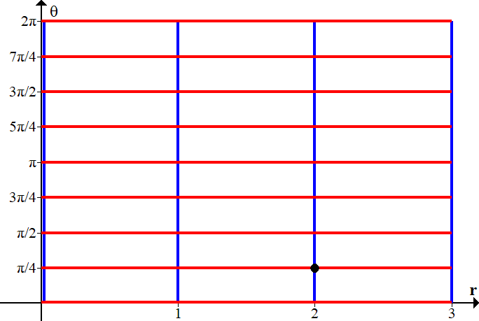
P → 
2. Specializing the Jacobian matrix in the above Notes to the point (r,θ) = (2,π⁄4) gives:
[DP(2,π⁄4)] = cos(π⁄4) −2 sin(π⁄4) sin(π⁄4) 2 cos(π⁄4) = √2⁄2 −√2 √2⁄2 √2 3. The affine approximation function to P near the base point (r,θ) = (2,π⁄4) is:
A(r, θ) = P(2,π⁄4) + DP(2,π⁄4)(r-2, θ−π⁄4) = (√2, √2) + (√2⁄2(r-2) − √2(θ−π⁄4) , √2⁄2(r-2) + √2(θ−π⁄4)). The corresponding gridlines are c(θ) = A(2,θ), A(3,θ), and parallel lines; and c(r) = A(r,π⁄4), A(r,π⁄8), and parallel lines: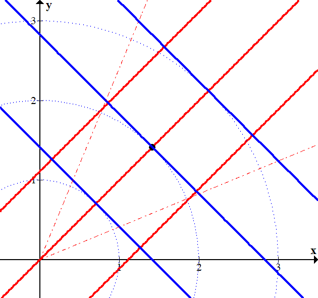
- 9/23 Lect 11. ⊞ Parametrizing a region R as F(u,v) for (u,v) ∈ R*
⊞ Solutions- To parametrize a region R in the (x,y)-plane, we find an adapted mapping F : R2 → R2 of the form F(u,v) = (x(u,v), y(u,v)), and a simple parameter region R* in the (u,v) plane, usually a rectangle, such that F maps R* onto R.
- Example: The polar mapping P(u,v) = (u cos(v), u sin(v)) parametrizes the unit circle R by the parameter rectangle R* = [0,1] × [0,2π], i.e. (u,v) with 0 ≤ u ≤ 1, 0 ≤ v ≤ 2π.
- Parametrize a triangle
- Consider a (u,v)-grid in the (x,y)-plane
R2 whose u-lines (red) are
parallel to the vector (2,1), and whose v-lines (blue)
are parallel to (1,3).
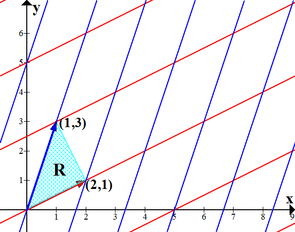
- Consider the triangular region R (light blue) with vertices (0,0), (2,1), (1,3). Find a triangular parameter region R* in the (u,v) plane which is taken to R by the mapping L: that is, L parametrizes R by R*. (Define R* in terms of inequalities such as u ≥ 0 and v ≤ f(u) for some function f.)
- Now let R be any triangular region in the (x,y) plane with vertices a, b, c. Generalize the above exercise to define an affine linear function F(u,v) and a parameter region R* which parametrize R. (It may be convenient to define F(u,v) in terms of the vectors b−a, c−a, rather than in coordinates.)
- Consider a (u,v)-grid in the (x,y)-plane
R2 whose u-lines (red) are
parallel to the vector (2,1), and whose v-lines (blue)
are parallel to (1,3).
- Inversion mapping
- Let F : R2 → R2 be the mapping which takes a non-zero vector (u,v) to a vector (x,y) with the same direction and the reciprocal radius: that is, F turns the unit circle "inside out" so that its interior is stretched to cover the whole plane outside the circle, and region outside the circle is squashed inside. Find a vector formula for F(v), as well as a coordinate formula F(u,v) = (x,y).
- Sketch the F(u,v)-grid produced by the above mapping in the (x,y)-plane. Hint: The integer grid lines in the (u,v) plane are all taken to small circles inside the unit circle. Since each (u,v)-grid line goes to infinity in the (u,v)-plane, its image goes to the origin in the (x,y)-plane. These are called Apollonian circles.
- Extra Credit: Inverting familiar curves in the (u,v) plane gives interesting new curves in the (x,y) plane. The inversion of the parabola v = u2 − 1 is called the cardioid: you can parametrize it as c(u) = (x(u), y(u)) = F(u, u2−1). Similarly, the inversion of the hyperbola u2 − v2 = 1 is called the lemniscate of Bernoulli. Explore these curves, and say as much as you can about them, showing how the inversion definition is equivalent to the usual ones you can find online. For example, find (x,y) equations defining these curves, or polar coordinate equations r = f(θ). Does the inversion mapping give insight on their properties?
- Parametrizing rotated objects
- Parametrize the region R bounded by the ellipse x2⁄4 + y2⁄9 = 1. That is, find a function F(u,v) which takes some simple (u,v)-region R* to R. Hint: The extreme points of the ellipse are (±2,0) and (0,±3). Stretch the x and y coordinates of the usual polar parametrization of the unit disk to get the correct height and width.
- Now parametrize the same ellipse, but rotated 45° and with its center shifted to (1,2). Hint: Take the the previous parametrization mapping, then compose it with rotation and translation mappings.
1a. We just need the (u,v) coordinate axis vectors to map as L(i) = (2,1) and L(j) = (1,3), and the rest of the grid follows. Thus L(u,v) = (2,1)u + (1,3)v = (2u+v, u+3v). Note that the matrix of L is [
].2 1 1 3 1b. The parameter region is the standard triangle with vertices (u,v) = (0,0), (1,0), (0,1). That is, R* = {(u,v) with 0 ≤ u and 0 ≤ v ≤ 1−u} = {(u,v) with u ≥ 0, v ≥ 0, u+v ≤ 1}.
1c. F(u,v) = a + (b−a)u + (c−a)v will take the standard (u,v) grid to the grid generated by the edge-vectors b−a and c−a, with the origin taken to a. Use the previous parameter region R* = {(u,v) with u ≥ 0, v ≥ 0, u+v ≤ 1}.
2a. The vector parallel to v = (u,v), having length 1⁄|v|, is F(v) = v⁄|v|2, which means F(u,v) = ( u⁄u2+v2 , v⁄u2+v2 ).
2b. To see the transformation of the (u,v) grid under the mapping F(u,v), apply a parametric curve plotter successively to c(t) = F(1,t), F(2,t), F(3,t) gives red circles labeled u = 1,2,3 with diameter 1, 1⁄2, 1⁄3, all passing through the origin and with centers on the y-axis. Similarly for blue circles c(t) = F(t,1), F(t,2), F(t,3) centered on the x-axis.

3a. F(r,θ) = (1⁄2 r cos(θ), 1⁄3 r sin(θ)) over the region (r,θ) ∈ R* = [0,1]×[0,2π].
3b. The rotation map Rotπ⁄4 is defined by a rotation matrix which works out to Rot(x,y) = 1⁄√2(x+y, x−y). Applying this to the output of the previous F(r,θ), then translating by (1,2), gives:
G(r,θ) = ( 1 + r⁄2√2 cos(θ) + r⁄3√2 sin(θ) , 2 + r⁄2√2 cos(θ) − r⁄3√2 sin(θ) ). Here we should think of r as measuring an "elliptically scaled" radius measured from the center of the tilted, translated ellipse; and θ as measuring a squashed "elliptical angle".- 9/25-27 Lect 12-13. ⊞ Product and Chain Rules
Soln- Theme: Close up, any smooth function looks like an affine linear function.
- Product Rule: To find derivative of product, multiply affine approx
∇(fg)(a) = f(a) ∇g(a) + ∇f(a) g(a) - Chain Rule for f,g : R → R, compose affine approximations:
f(g(a+h)) ≈ f( g(a) + g'(a)h ) ≈ f(g(a)) + f '(g(a)) g'(a)h
So: (f(g(t)))' = f '(g(t)) g'(t) , d⁄dt(f(g(t))) = df⁄dx(g(t)) dg⁄dt(t)
Ex: d⁄dt(sin(t2)) = sin'(t2) (t2)' = cos(t2) 2t - Chain Rule for f : R2 → R ,
c : R → R2 ,
c(t) = (x(t), y(t)) ,
f∘c : R → R,
f(c(a+h)) ≈ f( c(a) + c'(a)h ) ≈ f(c(a)) + ∇f(c(a)) • c'(a)h
So: d⁄dtf(g(t)) = ∇f(c(t)) • c'(t) = ∂f⁄∂xdx⁄dt + ∂f⁄∂ydy⁄dt
Ex: f(x,y) = sin(xy) , c(t) = (x(t),y(t))= (t2, t+1) , f(c(t)) = sin(t2(t+1))
d⁄dt sin(t2(t+1)) = ∇sin(xy) • d⁄dt(t2, t+1)
= (cos(xy) y , cos(xy) x) • (2t, 1)
= cos(xy) (x(2t) + y(1)) = cos(t2(t+1)) (2t3+t+1) - Chain Rule for
F,G : R2 → R2
Compose affine approximations: D(F∘G)a(h) = DFG(a)( DGa(h) )
Multiply Jacobian matrices: [D(F∘G)a] = [DFG(a)] • [DGa]
Ex: L(x,y) = Shear(x,y) = (x+y, y), P(r,θ) = (r cos(θ), r sin(θ)) = (x,y) ,
L(P(r,θ)) = (r(cos(θ)+sin(θ)), r sin(θ)) sheared polar coord map
[D(L∘P)(r,θ)] = [DL(x,y)] • [DP(r,θ)] = [L] • [DP(r,θ)], multiply Jacobian matrices
HW: Look at WHW 5 due 9/30 below.- For a function F : Rn → Rm and a center point a ∈ Rn, we define the derivative DFa to be the linear function which gives the best affine approximation for x ≈ a: that is, F(a+h) ≈ F(a) + DFa(h). Show that if F = L is itself a linear function, then DLa = L at any a. That is, a linear function has a constant Jacobian matrix of slopes.
- Given a function f(x,y), its polar coordinate form is g(r,θ) = f(r cos(θ), r sin(θ)). Find the gradient ∇g(r,θ) using the Chain Rule.
- First, use the matrix form of the Chain Rule, multiplying the gradient of f(x,y) by the Jacobian matrix of the polar coordinate map P(r,θ).
- Redo this using the letter-form of the Chain Rule:
for z = f(x,y), x = r cos(θ), y = r sin(θ),
we have:
∂z⁄∂r = ∂z⁄∂x ∂x⁄∂r + ∂z⁄∂y ∂y⁄∂r , and similarly for ∂z⁄∂θ.
- A polar graph is a curve around the origin in which the radius is a function of the angle: r = r(θ). That is, the curve c(t) = P(r(θ), θ), where P(r,θ) is the polar coordinate mapping. Use the Chain Rule to compute the tangent vector of this curve at a given value of θ.
- Given functions f,g : R2 → R, we showed the Product Rule for ∇(fg)
by multiplying linear approximations. Here is another proof, assuming the Chain Rule.
Consider the multiplication function m(x,y) = xy, and F(x,y) = (f(x,y), g(x,y)), where F : R2 → R2. Then we can write the product function as: f(x,y) g(x,y) = m(F(x,y)). Compute the derivative matrices [∇m] and [DF], and apply the Chain Rule to deduce the derivative of the product. - Given f,g : R2 → R, find the gradient (derivative) of h(x,y) = f(x,g(x,y)). Hint: Write h(x,y) as a composite of f(x,y) and a function G : R2 → R2.
- 9/26 Recitation 5. Parametrization, affine approx, Jacobian, WHW 5.
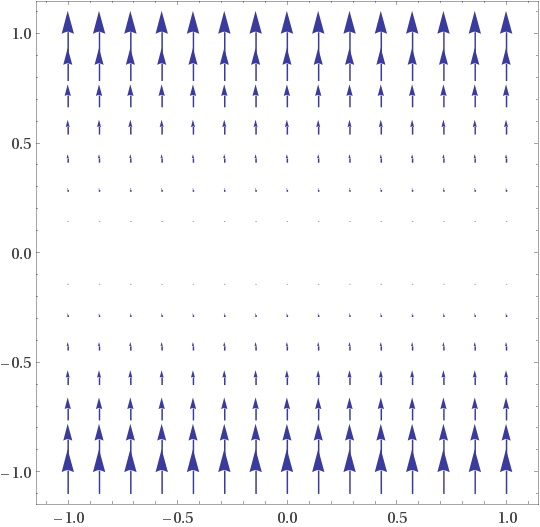
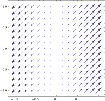
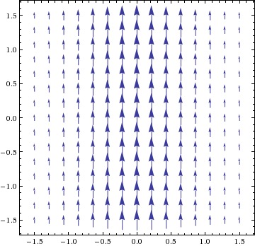
- 9/30 Lect 14. ⊞ Vector field F(x,y): grad & non-grad fields.
⊞ Solutions- Vector field: F : R2 → R2, F(x,y) = (p(x,y), q(x,y))
F(x,y) = arrow drawn at point (x,y), field of wheat stalks
Same data as F(u,v) = (x,y) motion of plane, different geometric meaning
Vector field plotter - Gradient vector field F(x,y) = ∇f(x,y)
⇒ draw contour map, level curves f = n
Gradient arrows are perpendicular to level curves, cutting straight across them
Proof: Parametrized level curve c(t) has f(c(t)) = const for all t
So d⁄dtf(c(t)) = (const)', by Chain Rule ∇f(c(t)) • c'(t) = 0
So gradient vector orthogonal to level curve tangent vector
Distance d between level curves f = n and f = m:
|∇f| = slope between level curves = rise⁄run ≈ (m−n)⁄d, so d ≈ (m−n)⁄|∇f| - Ex: F(x,y) = ∇(x2+y2) = (2x,2y), F(v) = 2v
vanishes at (0,0), radial, gets longer outward
F(x,y) = (0,y), vertical vectors ⇒ horiz level curves, F(x,y) = ∇(y2) trough function
F(x,y) = (y,0), horiz vectors, river with no flow on x-axis, opposite flows above & below
If F = ∇f level curves vertical, but uphill arrow inconsistent, so F not gradient
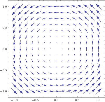
F(x,y) = (−y,x), F(v) = v⊥ turn-table velocity field, circular flows
F ≠ ∇f: level curves radial, values inconsistent at different radii
HW:- Rectangular vector fields.
Sketch the following by hand.
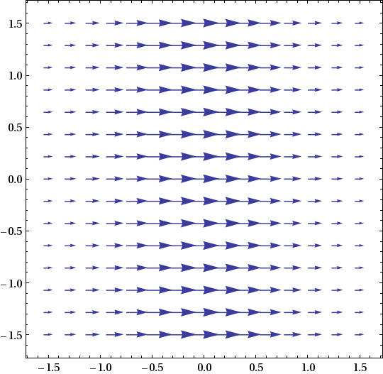
- F(x,y) = 2i + j = (2,1), constant arrows
- F(x,y) = sin(x) j = (0, sin(x)), vertical arrows with length oscillating as (x,y) moves horizontally
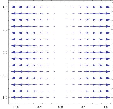
- F(x,y) = cos(x) i = (cos(x), 0), horizontal arrows with length oscillating as (x,y) moves horizontally
- F(x,y) = cos(x) i + sin(x) j = (cos(x), sin(x)), unit arrows rotating as (x,y) moves horizontally
- Which of the above could be gradient fields? If so, find f(x,y) with F = ∇f. If not, find an inconsistency involving possible contour lines.
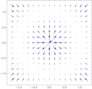
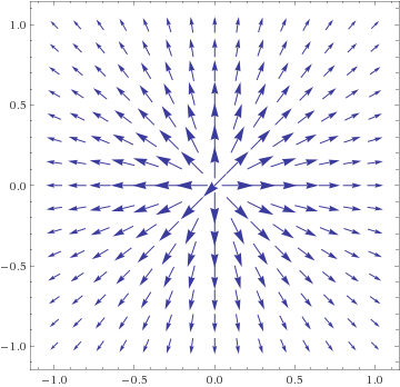
- Polar vector fields (radial + circular).
Sketch the following by hand.
Notation: v = (x,y), v⊥ = (−y,x) = 90° rotation of v.- F(v) = v⁄|v| unit-length radial
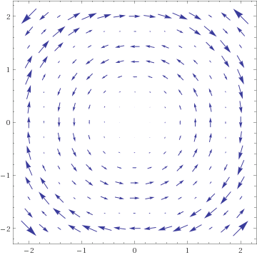
- F(v) = v⊥⁄|v| unit-length circular
- F(v) = v⊥⁄|v| − v⁄|v| whirlpool
- For each pictured vector field, give a formula which produces the picture, at least approximately.
-
- Find the unique circular vector field F(v) = g(|v|) v⊥ which is a gradient, F(v) = ∇f, at least in most of the plane. Try to draw the contour map and imagine the graph of f(x,y). Hint: the total circular gradient flow between two radial contour lines must be the same for any radius: this determines the magnitude.
1,2. Use the vector field plotter to check your sketches. Some principles: Know a few basic vector fields, such as constant fields F = i, j radial field F(v) = v, rotation field F(v) = v⊥; how to scale (stretch) them by given functions f(x) and f(y); and how to combine them by adding the vectors at each point. Given a formula for F, build it up from simple fields by known operations.3a. Vertical, so (0, g(x,y)), length depends only on height, so (0, g(y)). Ans: F(x,y) = (0, y2) = ∇(0, ⅓y3)
3b. Clearly g(x,y) (1,1), length depends only on x, so g(x) (1,1). Ans: F(x,y) = x(1,1) = (x,x)
3c. Radial unit length would be F(v) = v⁄|v|. To adjust length by radius, scale: g(|v|) v⁄|v|. Here, g(0) = 1, g(1) = 0, g(r) < 0 for r > 1; take g(r) = 1−r. Ans: (1−√(x2+y2)) (x,y)⁄√(x2+y2) .
4. To have consistent circular flows, the circular gradient field must have magnitude |F(v)| = 1⁄|v|, so take g(|v|) = 1⁄|v|2. Then z = f(x,y) has radial level curves, and is a helical staircase surface, in which the height of a radial line equals its polar angle: f(x,y) = θ = arctan(y⁄x), at least for x > 0.
- 10/2 Lect 15. ⊞ Path independence, circulation, curl F.
⊞ Solutions- Potential: We say a vector field F(x,y) is conservative if it has a potential function f(x,y) with ∇f = F, which is not always possible.
- If F is conservative, it has the same line integral for any curve c between two given points, such as (0,0) and (a,b), since the Gradient Theorem tells us ∮ F(c)•dc = f(a,b) − f(0,0). We say that F is path-independent.
- The line integral around a closed curve c,
a loop with c(0) = c(1), is called the
circulation of F around the loop.
(This is the reason for the little circle in the ∮ symbol.)
Let F be path independent. We can cut the loop c(t) into two halves, both from c(0) to c(½): namely c1(t) = c(t) and c2(t) = c(1−t) for 0 ≤ t ≤ ½, the second going backward from the end of loop. By path independence:∮ F(c)•dc = ∮ F(c1)•dc1 − ∮ F(c2)•dc2 = 0. We say that F has zero circulation. - Curl: The easiest way to measure whether F is conservative is to compute its rate of circulation at each point
(x,y).
We define the scalar function
(curl F) : R2 → R
in terms of the partial derivatives of the components
of F = (p,q):
curl F(x,y) = ∂q⁄∂x − ∂p⁄∂y. Geometrically, curl F measures the rate of circulation of F around a point (x,y) = (a,b), relative to the area enclosed by the boundary loop:
curl F(a,b) = limR → (a,b) ( ∮ F(c) • dc ) / area(R) , where the limit is over smaller and smaller regions R containing (a,b), and c is the counterclockwise boundary curve of R.
If has zero circulation, we have curl F(x,y) = 0 for all (x,y), and we say F is irrotational. -
Example: The field F(x,y) = (0,
1⁄(1+x2))
could represent the velocity of a river flowing strongest along the middle (the y-axis):
We compute: curl F(x,y) = ∂⁄∂x(1⁄(1+x2)) − ∂⁄∂y(0) = −2x⁄(1+x2)2 , and we verify that curl F(1, 0) = −½, and F(−1, 0) = ½. -
We will later show that all the following are equivalent:
- F = ∇f is conservative, the gradient of a potential function.
- F is path independent: the line integral between any two points (a1,b1) and (a2,b2) does not depend on the path chosen, ∮ F(c1)•dc1 = ∮ F(c2)•dc2 for any c1, c2 from (a1,b1) to (a2,b1).
- F has zero circulation: around any closed curve c, a loop with c(0) = c(1), the line integral ∮ F(c)•dc = 0.
- F is irrotational: curl F = 0 at all (x,y).
HW: Start WHW 6 due 10/7.- For each of the following vector fields F:
- Sketch F, and visually estimate curl F, the rate of rotation at each point: this is how strongly a little paddlewheel would be turned counterclockwise around the point (x,y) in the flow given by F.
- For F(x,y) = (p(x,y), q(x,y)), compute curl F = ∂q⁄∂x − ∂p⁄∂y, and compare to your estimate.
- If curl F = 0 everywhere, meaning F is irrotational, find the potential function f(x,y) = ∮ F(c) • dc for c from (0,0) to (x,y), and check ∇f = F, showing that F is conservative.
- F(x,y) = (0, x)
- F(x,y) = (x, 0)
- The vortex field F(x,y) = (−y, x). Imagine sitting on a turntable, with your velocity given by F. To keep from getting dizzy, you turn your head toward a fixed point on the horizon. The curl is your head's rate of rotation.
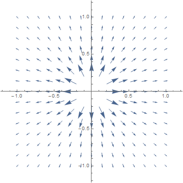
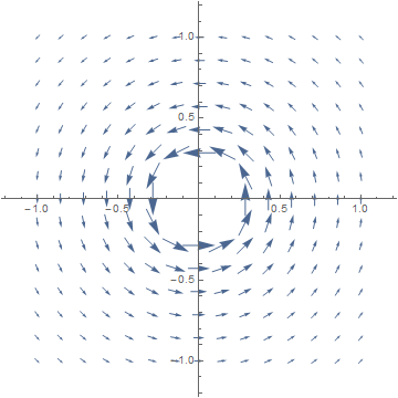
- Any radial field of the form F(x,y) = g(r) (x,y), where g(r) is any scalar function of the radius r = √(x2 + y2). For example g(r) = 1⁄r2 gives radial vectors of length inversely proportional to the distance from the center: F(x,y) = 1⁄(x2+y2) (x,y) = (x⁄(x2+y2) , y⁄(x2+y2)).
- Consider the rotational vector field with length
inversely proportional to the distance from the center:
F(x,y) = 1⁄(x2+y2) (−y, x) = (−y⁄(x2+y2) , x⁄(x2+y2)). - Verify that the length |F(x,y)| = 1/r. Sketch the vector field F, noting that it is undefined at the origin, and guess curl F.
- Show that curl F = 0 everywhere except at the origin. This means the rotation is all "concentrated in the center".
- Compute a potential function f(x,y) defined away from the negative x-axis, i.e. for any (x,y) with y ≠ 0 or x > 0.
Staying away from the singular point (0,0),
take a line integral along the radial line segment from (1,0) to (r,0),
then a circlar arc (r cos(t), r sin(t)) from (0,r) to (a,b),
where r = √(a2 + b2)
and t goes from 0 to arctan(b/a).
Note: The graph z = f(x,y) is a "spiral staircase" whose height equals the angle of (x,y) from the positive x-axis: z = θ. Can we define f(x,y) with ∇f = F for all (x,y) ≠ (0,0)?
1a. F(x,y) = (0, x)
A small paddlewheel placed at any point is pushed vertically on one side more than on the other, giving a counterclockwise rotational force, which means curl F > 0.
In fact, curl F = ∂⁄∂x(x) − ∂⁄∂y(0) = 1 − 0 = 1. Since the curl is non-zero, the field is not conservative, and cannot have a potential function f.1b. F(x,y) = (x, 0).
The equal flows on the top and bottom of a paddlewheel cancel each other, so we should have curl F = 0.
In fact, curl F = ∂⁄∂x(0) − ∂⁄∂y(x) = 0 − 0 = 0. The line integral along c(t) = (at, bt) is: f(a,b) = ∫01 F(at, bt) • (at, bt)' dt = ∫01 (at, 0) • (a, b) dt = ½a2. The potential function is thus f(x,y) = ½x2.1c. F(x,y) = (−y, x).
A paddlewheel is pushed harder on the side away from the origin than on the side facing the origin, giving a counterclockwise rotation, curl F > 0.
Using the other physical model, a person sitting anywhere on a turntable must turn his head at a constant rate to counter the table's rotation, so we expect curl F is constant.
In fact, curl F = ∂⁄∂x(x) − ∂⁄∂y(−y) = 1 − (−1) = 2. There is no potential function.1d. F(x,y) = 1⁄r2 (x,y).
We compute: r = √(x2+y2), ∂r⁄∂x = x⁄√(x2+y2), and similarly for ∂r⁄∂y, so the Chain Rule gives:curl F = ∂⁄∂x [g(r) y] − ∂⁄∂y [g(r) x]
= g'(r) x⁄√(x2+y2) y − g'(r) y⁄√(x2 +y2) x = 0.The potential function is f(x,y) = r G(r), where G(c) = ∫c0 g(r) dr.
2a. The magnitude of F(x,y) = 1⁄r2 (−y, x) is |F(x,y)| = 1⁄r2 |(−y, x)| = 1⁄r2 r = 1⁄r .
On the side away from the center, a paddlewheel is pushed counterclockwise by the flow; on the side facing the center, it is pushed clockwise along a shorter arc by a stronger flow. The two forces balance, and we should have curl F = 0.
2b. For F(x,y) = (−y⁄x2+y2 , x⁄x2+y2), we use the Quotient Rule to get:
curl F = ∂⁄∂x(x⁄x2+y2) − ∂⁄∂y(−y⁄x2+y2)
= (x2 + y2 − x(2x))⁄(x2+y2)2 − (−x2 − y2 − (−y)(2y))⁄(x2+y2)2 = 0That is, F has no rotation at any point where it is defined, though it has some singular behavior at the origin.
2c. To compute the potential function f(a,b), we take the line integral along a two-segment path: we define the constant s = √(a2+b2), and take the line segment c1(t) = (t + (1−t)s, 0) from (1,0) to (r,0); then the circular arc c2(t) = (s cos(t), s sin(t)) from (r,0) to (a,b), where t goes from 0 to θ = arctan(b/a), which is the angle from the x-axis to the radial vector (a,b). The potential function is given by:
f(a,b) = ∮ F(c1) dc1 + ∮ F(c2) dc2
= ∫01 F(st, 0) • (st,0)' dt + ∫0θ F(s cos(t), s sin(t)) • (s cos(t), s sin(t))' dt
= ∫01 1⁄r2(0, st) • (s,0) dt + ∫0θ 1⁄s2(−s sin(t), s cos(t)) • (−s sin(t), s cos(t)) dt
= 0 + ∫0θ s2⁄s2 (sin2(t) + cos2(t)) dt = θ = arctan(b/a).
In the graph z = f(x,y), the ray at angle θ from the x-axis is at height θ, for −π ≤ θ ≤ π. This leads to a discontinuity on the negative x-axis, where the angle can be either π or −π. Thus, we cannot define the potential function all the way around the origin, which reflects the fact that F does have a rotation around that point, though nowhere else.
- 10/3 Recitation 6. Mean Value Theorem and two definitions of curl, WHW 6.
- 10/4 Lect 16. ⊞ Flux ∮F•dn & div F.
⊞ Solutions- Flux integral. The flux of a vector field F across a curve c is the net flow of F from the left to the right side of c, facing forward along the curve.
-
By this we mean that c(t) = (x(t), y(t))
has velocity vector c'(t) = (x'(t), y'(t)),
whose counterclockwise orthogonal
c'(t)⊥ = (−y'(t), x'(t))
points to the left side of c; and
the right-side orthogonal n(t) = −c'(t)⊥
= (y'(t), −x'(t)) is called the normal vector.
To see how strongly the field F is flowing across the curve c at a given point, we take the the dot product of F(c(t)) • n(t) The flux is the line integral of this quantity:Flux = ∮ F(c) • dn = ∮ F(c) • (−dc⊥) = ∫10 F(c(t)) • (−c'(t)⊥) dt. As with the circulation integral, we can also define flux (and compute it numerically) as a Rienmann sum:
∮ F(c) • dn = limn→∞ ∑ i=0 n−1 F(ci) • (−Δci⊥), where we take sample points c0, . . . ,cn on the curve c, and Δci = ci+1−ci ≈ c'(ti) Δti . - Divergence: For a vector field F on the xy-plane,
we define its divergence as the rate
of outflow of F from a small region near (x,y) = (a,b),
relative to the area of the region:
div F(a,b) = limΔx,Δy → 0 ( ∮ F(cΔxΔy) • dn ) / ΔxΔy , where cΔxΔy(t) is the curve which traces counterclockwise around a rectangle from (a,b) to (a+Δx, b) to (a+Δx, b+Δy) to (a, b+Δy) and back to (a,b), and dn(t) = −dcΔxΔy(t)⊥ is the outward normal vector of the rectangle.
The above limit can be computed to give a formula in terms of the partial derivatives of the components of F(x,y) = (p(x,y), q(x,y)):div F(x,y) = ∂p⁄∂x + ∂q⁄∂y . If div F(x,y) = 0 everywhere, we say F is incompressible, modeling velocity of a fluid in which there is no net outflow from any region. - Example: The field F(x,y) = (1⁄(1+x2), 0)
could represent the velocity of the Red Cedar River flowing over
the dam (the y-axis): the river gets faster where it is shallower.
We compute: div F(x,y) = ∂⁄∂x(1⁄(1+x2)) − ∂⁄∂x(0) = −2x⁄(1+x2)2 , and we verify that div F(−1, 0) = ½. Similarly, F(1, 0) = −½.
HW: Finish WHW 6 due 10/7 below.- Picturing divergence (compare Lect 13 #1). For each of the following vector fields F:
- Sketch F, and visually estimate div F, the rate of outflow at each point (x,y).
- For F(x,y) = (p(x,y), q(x,y)), compute div F = ∂p⁄∂x + ∂q⁄∂y, and compare to your estimate.
- F(x,y) = (0, x)
- F(x,y) = (x, 0)
- The radial field F(x,y) = (x,y).
- A rotational field F(x,y) = g(r) (−y, x), where g(r) is any scalar function of the radius r = √(x2 + y2). For example g(r) = r−2, giving F(x,y) = (−y⁄(x2+y2) , x⁄(x2+y2)).
- Consider the radial vector field with length
inversely proportional to the distance from the center:
F(x,y) = 1⁄(x2+y2) (x,y) = (x⁄(x2+y2) , y⁄(x2+y2)). - Verify that the length |F(x,y)| = 1/r. Sketch the vector field F, noting that it is undefined at the origin, and guess div F.
- Show that div F = 0 everywhere except at the origin, meaning F is incompressible. This means the divergence is all "concentrated in the center".
- Compute the flux integral (total outflow) ∮c F • dn across the boundary curve c of the polar-box region D defined by 0 ≤ r ≤ 1, 0 ≤ θ ≤ π⁄2. Verify that it is indeed zero.
1a. F(x,y) = (0,x)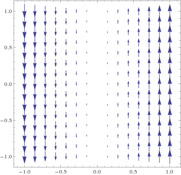
1b. F(x,y) = (x,0)
1c. F(x,y) = (x,y)

1d. F(x,y) = sin(x2+y2) (−y,x)
div F = ∂⁄∂x(g(x2+y2)(−y)) + ∂⁄∂y(g(x2+y2)x)
= g'(x2+y2)(2x)(−y) + g'(x2+y2)(2y)(−x) = 02a. F(x,y) = (x⁄(x2+y2) , y⁄(x2+y2)). A rough sketch, with the large vectors near the origin not show to scale:
For any small radial box, the radial edges have zero flow; and the inner circular edge has a shorter arc with longer inflowing F vectors, while the outer circular edge as a longer arc with shorter outflowing F vectors. Thus we may guess div F ≈ 0 everywhere (except at the origin, where there is a positive outflow from zero area, an infinite rate of outflow).
2b. Compute for radial field F(x,y) = g(x2+y2) (x,y) = 1⁄(x2+y2) (x,y):
div F = ∂⁄∂x(g(x2+y2)x) + ∂⁄∂y(g(x2+y2)y) 2c. The radial box consists of curves:
= g'(x2+y2)(2x2) + g(x2+y2) + g'(x2+y2)(2y2) + g(x2+y2)
= −2(x2+y2)⁄(x2+y2)2 + 2⁄(x2+y2) = 0.c1(t) = (t+1, 0) , c2(t) = (2 cos(π⁄4 t), 2 sin(π⁄4 t)), where all parameters run over 0 ≤ t ≤ 1. These have tangent vectors:
c3(t) = (0, 2−t) , c4(t) = (cos(π⁄4(1−t)), sin(π⁄4(1−t))),c'1(t) = (1,0) , c'2(t) = (−π⁄2 sin(π⁄4 t), π⁄2 cos(π⁄4 t)), Since n(t) = −c'(t)⊥, where −(x,y)⊥ = (y,−x), we have:
c'3(t) = (0,−1) , c'4(t) = (π⁄4 sin(π⁄4(1−t)) , −π⁄4 cos(π⁄4(1−t))).n1(t) = (0,−1) , n2(t) = (π⁄2 cos(π⁄4 t), π⁄2 sin(π⁄4 t)), The flux integral is a sum of four line-integrals over c1, c2, c3, c4, for example:
n3(t) = (−1,0) , n4(t) = (−π⁄4 cos(π⁄4(1−t)) , −π⁄4 sin(π⁄4(1−t))).∮ c2 F(c2(t)) • dn2 = ∫01 F(2 cos(π⁄4 t), 2 sin(π⁄4 t)) • (π⁄2 cos(π⁄4 t), π⁄2 sin(π⁄4 t)) dt Note this is positive because there is a net outflow across c2: that is, F(c2(t)) flows from left to right, facing along c'2(t). Similarly, the integral for c4 is −π⁄2 , and the other two integrals are both zero, since F is orthogonal to the normal.
= ∫01 (1⁄2 cos(π⁄4 t), 1⁄2 sin(π⁄4 t)) • (π⁄2 cos(π⁄4 t), π⁄2 sin(π⁄4 t)) dt = π⁄2 .
- 10/7 Lect 17. ⊞ Double integral ∬D f(x,y) dx dy
⊞ Solutions- Arclength of c(t) = (x(t),y(t))
for a ≤ t ≤ b:
L = limn→∞ ∑ i=0 n−1 |Δci| = limn→∞ ∑ i=0 n−1 |Δc'(ti)| Δti Length is integral of speed (abs value of velocity).
= ∫ab |c'(t)| dt = ∫ab √(x'(t)2+y'(t)2) dt . - Double integral is volume below graph z = f(x,y),
above planar domain D.
For rectangle domain:D = [a,b]×[c,d] = {(x,y) with a ≤ x ≤ b , c ≤ y ≤ d}, take sample points in x-interval and y-interval:a = x0 < x1 < ··· < xn = b Sum up volumes of "french fries" above n×n tiny rectangles at (xi,yj):
c = y0 < y1 < ··· < yn = d.
volume is: height f(xi,yj), times base area Δxi Δyj.∬D f(x,y) dx dy = limn→∞ ∑ i,j=0 n−1 f(xi,yj) Δxi Δyj . We can equally well write dy dx instead of dx dy. - Cavalieri Principle: To compute volume, integrate areas of all slices perpendicular to an axis.
Fubini Theorem: To compute double integral ∬D f(x,y) dx dy,- Evaluate area of each slice perpendiuclar to y-axis: the inside integral A(y) = ∫ab f(x,y) dx with respect to x-variable, considering y as constant.
- Integrate ∫cd A(y) dy along y-axis.
- Can also switch to dy dx, do y-integral first.
-
Example: Rectangular region D = [0,1]×[2,3] with 0 ≤ x ≤ 1 and 2 ≤ y ≤ 3,
function f(x,y) = xy2, we have:
∬D xy2 dx dy = ∫32 (∫10 xy2 dx) dy
= ∫32 [1⁄2x2y2]x=0 x=1 dy = ∫32 1⁄2y2 dy = 19⁄6 .∬D xy2 dy dx = ∫10 (∫32 xy2 dy) dx
= ∫10 [1⁄3xy3]y=2 y=3 dy = ∫10 1⁄3(27x − 8x) dx = 19⁄6 .
HW:- Arclength
- Find the arclength of the graph y = x2 for 0 ≤ x ≤ 1. Hint: Recall the integral formula ∫√(a2+x2) dx = x⁄2√(a2+x2) + a2⁄2 log(x+√(a2+x2)) + C.
- Using our formula for parametrized curves, derive the formula for arclength of a graph y = f(x) over a ≤ x ≤ b.
- Recall the cycloid curve c(t) = (t−sin(t), 1-cos(t)), the path of a point on the rim of a rolling wheel. Find the length of one arch of the curve, from t = 0 to t = 2π. Hint: Use a trig half-angle formula to evaluate the integral.
- A bunch of double integrals, done both ways (dx dy and dy dx):
[MT] Ch 5.1 p 269, Ex #1,2,3,4. Ch 5.2 p 282, Ex #1. - Sketch the solid region whose volume is computed by
the given integral.
- ∬R x+y2 dx dy for R = [0,1]×[−1,1]
- ∬R 1+xy dx dy for R = [0,2]×[0,3]
1a. Parametrize the curve as c(t) = (t,t2) for 0 ≤ t ≤ 1, giving length L = ∫10 √(12 + (2t)2) dt = 1⁄2√5 + 1⁄4log(2+√5). Even quite simple curves give difficult arclength integrals, which can usually only be evaluated numerically.1b. Parametrize as c(t) = (t, f(t)) for a ≤ t ≤ b, with c'(t) = (1, f '(t)), and length L = ∫ba √(1+f '(t)2) dt.
1c. See [MT] Ch 4.2 Example 2, p 229.
2. See [MT] answers, p 517, or evaluate (indefinite or definite) double integrals using Wolfram. Note that doing an integral as dx dy or as dy dx should give the same answer.
3a. The solid is under the graph z = x+y2 and above the rectangle (x,y) ∈ [0,1]×[−1,1]. To visualize the graph, consider the slice above the x-axis (y=0), which is just the line z = x; and the slices perpendicular to the x-axis, above x = c, which are parabolas z = c+y2 rising from the backbone above the x-axis. See the graph in Wolfram.
3b. The graph is a saddle surface, with upward parabola above y = x, downward parabola above y = −x, and two flat lines above the x and y axes.
- 10/9 Lect 18. ⊞ Computing double integrals.
- Definition of ∬D f(x,y) dx dy for general domain D:
In Riemann sum, add only the sample points (xi,yj) ∈ D - Simple domains: generalize (x,y) ∈ D = [a,b] × [c,d]
x-simple D = {(x,y) | a ≤ x ≤ b , c(x) ≤ y ≤ d(x)}
y-simple D = {(x,y) | c ≤ y ≤ d , a(y) ≤ x ≤ b(y)} - Ex: D triangle bounded by y = x , y = 1−x , y = 0.
∬D x2+y2 dy dx
= ∫ x=0 x=1/2 ∫ y=0 y=x x2+y2 dy dx + ∫ x=1/2 x=1 ∫ y=0 y=1−x x2+y2 dy dx
∬D x2+y2 dx dy = ∫ y=0 y=1/2 ∫ x=y x=1−y x2+y2 dx dy
- Ex: D bounded between y = 2x2 and y = x2−2x+3
- Technique: Reversing the order of integration
∫ x=a x=b ∫ y=c(x) y=d(x) f(x,y) dy dx ⇒ sketch x-simple D
⇒ convert to y-simple D: y-shadow c ≤ y ≤ d
for given y, find x-floor and ceiling a(y) ≤ x ≤ b(y)
⇒ ∫ y=c y=d ∫ x=a(y) x=b(y) f(x,y) dx dy - More general: parametrized domain F : D* → D,
F(u,v) = (x,y)
Polar parametrization P(r,θ) = (r cos(θ), r sin(θ))
P(r,θ) stretches sample box Δθ Δr to polar grid box of area r Δθ Δr
(since arc of Δθ radians has length r Δθ).
∬D f(x,y) dx dy = ∬D* f(r cos θ, r sin θ) r dθ dr.
5.4 Changing the order of integration
HW: [MT] p. 288 and 293 odd exercises (answers p 518).
- Gaussian integral
I =
∫
−∞
∞
e−x2 dx.
The integrand e−x2
is the
or bell-curve or normal distribution
which gives the relative probability of a
random variable x with expectation value zero. (For example, x could be the height
of a randomly chosen woman, minus the average height.)
To make this a true probability distribution, we must scale it so that the total probability (the integral) is equal to one. That is, we must divide by the value of the integral I, but this is difficult to compute since e−x2 has no elementary anti-derivative. We outline an amazing solution using double integrals and change of coordinates.- Compute the double integral of e−(x2+y2) over the disk x2 + y2 ≤ R2, for a fixed radius R, and find the limit as R → ∞. Use the polar coordinate substitution: ∬D f(x,y) dx dy = ∬D* f(r cos θ, r sin θ) r dθ dr.
- Show that the integral of e−(x2+y2) over the rectangle [−R,R]×[−R,R] is equal to ( ∫ −R R e−x2)2 dx = I2.
- Compare the integral in (a) with that in (b), letting R → ∞, and compute the original integral I.
Solution: See M&T p. 332.
- 10/10 Recitation 7. Start WHW 7 due 10/14, computing double integrals.
- 10/11 Lect 19. ⊞ Det[L] = area, substitution ∬D f(x,y) dx dy = ∬D* f(F(u,v)) |DF| du dv
⊞ Solutions- Area stretching factor for linear L(u,v) is determinant
Defined by L(1,0) = u = (a,b) , L(0,1) = v = (c,d).
Stretching factor is area of parallelogram D with edges u,v
Area = base×height = |u| |v| sin θ(u,v)
= |u⊥| |v| cos θ(u⊥,v) = u⊥•v = −bc+ad = ad−bc for u⊥ = (−b,a)
Positive area if v counterclockwise from u, negative area if clockwise= det[L] = det(u,v) = det a c b d = ad − bc
Properties of det(u,v): bilinear, alternating det(u,v) = −det(v,u) ⇒ formula - Substitution Rule for 1-variable integrals: x = g(u)
Local stretching factor: dx = g'(u) du = dx⁄du du
∫ f(x) dx = ∫ f(g(u)) g'(u) du - Substitution Rule for G(u,v) = (x,y),
one-to-one & onto G : D* → D
Local stretching factor is det of Jacobian matrix of derivatives∬D f(x,y) dx dy for = ∬D* f(x(u,v),y(u,v)) |det[DG(u,v)]| du dv. Leibnitz notation: |det[DG(u,v)]| = |∂(x,y)⁄∂(u,v)| - Tradeoff in using substitution (x,y) = G(u,v):
simplify region (x,y) ∈ D ⇒ (u,v) ∈ D*
but complicate integrand f(x,y) ⇒ f(x(u,v),y(u,v)) |∂(x,y)⁄∂(u,v)| - Ex: Polar P(r,θ) = (x,y) to parametrize roundish regions
Jacobian determinant:
= r cos2(θ) + r sin2(θ) = rdet[DP(r,θ)] = det ∇x(r,θ) ∇y(r,θ) = det cos(θ) −r sin(θ) sin(θ) r cos(θ)
for (x,y) ∈ D = disk of radius 1, parametrized by (r,θ) ∈ D* = [0,1]×[0,2π].∬D x2+y2 dx dy = ∬D* ( (r cos(θ))2 + (r sin(θ))2 ) |det[DP(r,θ)]| dr dθ Note: This is exactly half the volume of the enclosing cylinder under z = 1.
= ∫2π0 ∫10 r2 r dr dθ = ∫2π0 1⁄4 dθ = 1⁄4 2π = π⁄2 .
HW: Finish WHW 7 due 10/14.- Use an appropriate parametrization to find formulas for
the following quantities:
- The volume under an arbitrary surface of revolution z = f(r) = f(√(x2+y2)) and above a ring-shaped region with a ≤ r ≤ b. You probably saw the resulting formula in Calculus II: what was it called?
- The integral of an arbitrary f(x,y) over the elliptical region D defined by (x−1)2 + y2⁄4 ≤ 1
- The integral of f(x,y) over the triangle with vertices a = (1,1), b = (3,2), c = (2,4).
- Vector geometry of the determinant
- Consider vectors u = (a,b), v = (c,d), forming an angle from u to v given by α with −π ≤ α ≤ π (positive meaning counterclockwise). Let β be the angle from v to u⊥, the 90° counterclockwise rotation of u.
- Let D be parallelogram with vertices 0, u, v, u+v.
- Let area(u,v) be the area of D, counted positively if α ≥ 0, and negatively if α ≤ 0.
- The following properties of the area function are easy to see geometrically:
- Bilinear:
area(au1+bu2, v) =
a area(u1,v) + b area(u2,v)
area(u, cv1+dv2) = c area(u,v1) + d area(u,v2) - Skew-symmetric: area(u,v) = −area(v,u)
- Unit square: area(i,j) = 1, where i = (1,0) and j = (0,1)
- Bilinear:
area(au1+bu2, v) =
a area(u1,v) + b area(u2,v)
- p. 348 #15: Use an appropriate change of variables to compute the integral
∬B exp((y−x)⁄(y+x)) dx dy over the triangle B
with vertices (0,0), (1,0), (0,1).
- Consider the change of variables transformation (s,t) = T(x,y) = (y−x, y+x).
Find its matrix [T], and verify that:
s t = [T] • x y - Find the image region B* = T(B): this is a triangle with vertices T(0,0), T(1,0), T(0,1).
- Given (s,t) = (y−x, y+x), solve the two linear equations to get x,y in terms of s,t. Use this to write the inverse transformation U = T−1 with (x,y) = U(s,t). Write the matrix [U] and verify that [U]•[T] = I, the identity matrix. Also B = U(B*).
- Write the Change of Variables formula for our integral, transforming it by U to (s,t) variables over B*.
- Evaluate the integral.
- Consider the change of variables transformation (s,t) = T(x,y) = (y−x, y+x).
Find its matrix [T], and verify that:
- Routine practice from M&T.
- p. 304 #15(a,b). Do with rectangular coordinates, then again with polar.
- p. 305 #25. Do with rectangular coordinates, then again with coordinates (s,t) defined by (x,y) = s (1,0) + t (2,1).
- p. 305 #27, 37.
1. Use the polar parametrization P(r,θ), having Jacobian determinant det[DP] = r, and which maps the parameter region D* = [a,b]×[0,2π] to the ring-region D = {(x,y) | a2 ≤ x2+y2 ≤ b2}. The volume is:Vol = ∬D f(√(x2+y2)) dx dy = ∫ab ∫02π f(r) r dθ dr = ∫ab 2πr f(r) dr. This is the familiar "Shell Method Formula" for solids of revolution, usually justified by adding up thin cylindrical shells having perimeter 2πr, height f(r), and thickness dr.1b. The region D is an ellipse with center (1,0), height 1, and width 2, so it is parametrized by a shift and scaling of polar coordinates: E(u,v) = (x,y) = (1 + u cos(v), 2u sin(v)), over the parameter region D* = [0,1]×[0,2π]. This has Jacobian determinant:
= 2u cos2(v) + 2u sin2(v) = 2udet[DE(u,v)] = det ∇x(u,v) ∇y(u,v) = det cos(v) −u sin(v) 2sin(v) 2u cos(v) ∬D f(x,y) dx dy = ∫01 ∫02π f(1 + u cos(v), 2u sin(v)) 2u dv du. 1c. The given triangle D is half of a parallelogram with edge-vectors u = b−a = (2,1) and v = c−a = (1,3). We parametrize D by the affine linear mapping A(u,v) = a + L(u,v) with L(i) = u, L(j) = v, so that A(u,v) = (1+2u+v, 1+u+3v), over the triangular parameter region D* = {(u,v) | u,v ≥ 0, u+v ≤ 1}. The Jacobian determinant is:det[DA(u,v)] = det[L] = det 2 1 1 3 = (2)(3)−(1)(1) = 5. ∬D f(x,y) dx dy = ∫01 ∫01−v f(1+2u+v, 1+u+3v) 5 du dv. 2. We have the vectors u = (a,b), v = (c,d), the projection p of v on u, and the projection q of v on u⊥.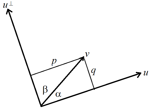
base×height = |u| |q| = |u⊥| |v| cos(β) = u⊥•v = (−b,a)•(c,d) = ac−bd. 3. Expand det(u,v) = det(a(1,0)+b(0,1), c(1,0)+d(0,1)) = ad-bc.4a. [T] = −1 1 1 1 4b. B* is the triangle with vertices (s,t) = (0,0), (−1,1), (1,1), given by 0 ≤ t ≤ 1, −t ≤ s ≤ t.
3c. (x,y) = (−½s + ½t , ½s + ½t). [U] = [T]−1 = −½ ½ ½ ½
This is indeed the inverse of [T], since: [U] • [T] = −½ ½ ½ ½ • −1 1 1 1 = 1 0 0 1 . 4d,e. We have U(B*) = B, one-to-one and onto. Since U is linear, it is its own derivative at every point: DU(s,t) = U, and |∂(x,y)⁄∂(s,t)| = det[U] = ½ . Also y−x = s, y+x = t. Thus:
∬B exp((y−x)⁄(y+x)) dx dy = ∬B* exp(s⁄t) |∂(x,y)⁄∂(s,t)| ds dt = 1⁄2 ∫01 ∫t−t es/t ds dt 5. See [MT] pp. 519−520
= 1⁄2 ∫01 ∫t−t es/t ds dt = 1⁄4 (e−e−1).
- 10/14 Lect 20. ⊞ Curl Theorem (Green's Thm) ∬S curl F dx dy = ∮ F(c)•dc
- One-variable Second Fundamental Theorem
Start with f(b)−f(a), break into small intervals ⇒ ∫ab f '(x) dx - Curl Theorem: The integral of the rate of circulation of a vector field F
over a region D is equal to the total circulation of
F around the boundary of D.
That is, letting c be the counterclockwise boundary curve of D, we have:
∬D curl F(x,y) dx dy. = ∮ F(c) • dc Justification: Start with the right-hand side, the circulation integral of F.
Break up into a double sum of circulations around sample grid boxes at (xi,yj),
where the line integrals over internal grid lines cancel, so the sum equals the boundary line integral.
Circulation around each box approaches curl F Δx Δy.
Limit of double sum over all i,j approaches double integral on left-hand side. - Example: Constant curl vector fields:
F(x,y) = (−y,0), (0,x), (−y,x)
Circulation around a loop equals (mult of) area enclosed
Start WHW 8 due Mon 10/21: Proof of Conservative Vector Field Theorem- 10/16 Lect 21. ⊞ Divergence Theorem (Green's Thm) ∬S div F dx dy = ∮ F(c)•dn
⊞ Solutions- Divergence Theorem (Green's Theorem for Flux):
For a vector field F,
the double integral of the rate of outflow of F over a region D
is equal to the total outflow of F across the boundary of D:
∬D div F dx dy = ∮ F(c) • dn . Here the closed curve c(t) = (x(t),y(t)) must not cross itself, and it must go counterclockwise enclosing D, a region with no holes or points where div F is undefined. Also recall that dn = (y(t),−x'(t)) dt is the outward-pointing normal vector at each boundary point.
The intuitive justification is that the flux line integral on the right side can be split over a grid of subregions at (xi,yj), whose flux integrals cancel each other along their common boundaries, except along the outside boundary of R. As the grid gets finer and finer, each small line integral near (xi,yj) is approximated by div F(xi,yj) Δx Δy, and their sum approaches the double integral on the left side. - Example: Consider F(x,y) = (1⁄(1+x2), 0) from Lect 16,
over the triangle region D, defined y-simply by 0 ≤ y ≤ 1 , 0 ≤ x ≤ 1−y.
The double integral of the rate of outflow (the divergence of F) over the region is:
∬D div F dx dy = ∫01 ∫0 1−y −2x⁄(1+x2)2 dx dy = ∫10 [1⁄1+x2 |1−y x=0 dy = ∫10 1⁄1+(1−y)2 − 1 dy = π⁄4 − 1.
The boundary of R consists of the line segments c1(t) = (t,0), c2(t) = (1−t,t), c3(t) = (0,1−t), each for 0 ≤ t ≤ 1; and the total flux is the line integral:
∮ F(c) • dn = ∮ F(c1) • dn1 + ∮ F(c2) • dn2 + ∮ F(c3) • dn3
= 0 + π⁄4 − 1 .In detail, one of these is:
∮ F(c2) • dn2 = ∫10 F(1−t, t) • (−(1−t, t)')⊥ dt Notice that n = (1,1) is the outward normal from the upper edge of the triangle.
= ∫10 (1⁄(1+t2), 0) • (−(−1,1)⊥) dt = ∫10 (1⁄(1+t2), 0) • (1,1) dt = π⁄4 .
HW: Continue WHW 8 due 10/21.- Consider the radial vector field with length
inversely proportional to the distance from the center:
F(x,y) = 1⁄(x2+y2) (x,y) = (x⁄(x2+y2) , y⁄(x2+y2)). - Verify that the length |F(x,y)| = 1/r. Sketch the vector field F, noting that it is undefined at the origin, and guess div F.
- Show that div F = 0 everywhere except at the origin, meaning F is incompressible. This means the divergence is all "concentrated in the center".
- Compute the flux integral (total outflow) ∮c F • dn across the boundary curve c of the polar-box region D defined by 0 ≤ r ≤ 1, 0 ≤ θ ≤ π⁄2. Verify that it is indeed zero: by the Divergence Theorem, the flux integral must equal the double integral of the rate of flux ∬D div F • dx dy, but div F = 0.
1a. F(x,y) = (x⁄(x2+y2) , y⁄(x2+y2)). A rough sketch, with the large vectors near the origin not show to scale:
For any small radial box, the radial edges have zero flow; and the inner circular edge has a shorter arc with longer inflowing F vectors, while the outer circular edge as a longer arc with shorter outflowing F vectors. Thus we may guess div F ≈ 0 everywhere (except at the origin, where there is a positive outflow from zero area, an infinite rate of outflow).
1b. Compute for radial field F(x,y) = g(x2+y2) (x,y) = 1⁄(x2+y2) (x,y):
div F = ∂⁄∂x(g(x2+y2)x) + ∂⁄∂y(g(x2+y2)y) 1c. The radial box consists of curves:
= g'(x2+y2)(2x2) + g(x2+y2) + g'(x2+y2)(2y2) + g(x2+y2)
= −2(x2+y2)⁄(x2+y2)2 + 2(x2+y2)⁄(x2+y2)2 = 0.c1(t) = (t+1, 0) , c2(t) = (2 cos(π⁄4 t), 2 sin(π⁄4 t)), where all parameters run over 0 ≤ t ≤ 1. These have tangent vectors:
c3(t) = (0, 2−t) , c4(t) = (cos(π⁄4(1−t)), sin(π⁄4(1−t))),c'1(t) = (1,0) , c'2(t) = (−π⁄2 sin(π⁄4 t), π⁄2 cos(π⁄4 t)), Since n(t) = −c'(t)⊥, where −(x,y)⊥ = (y,−x), we have:
c'3(t) = (0,−1) , c'4(t) = (π⁄4 sin(π⁄4(1−t)) , −π⁄4 cos(π⁄4(1−t))).n1(t) = (0,−1) , n2(t) = (π⁄2 cos(π⁄4 t), π⁄2 sin(π⁄4 t)), The flux integral is a sum of four line-integrals over c1, c2, c3, c4, for example:
n3(t) = (−1,0) , n4(t) = (−π⁄4 cos(π⁄4(1−t)) , −π⁄4 sin(π⁄4(1−t))).∮ c2 F(c2(t)) • dn2 = ∫01 F(2 cos(π⁄4 t), 2 sin(π⁄4 t)) • (π⁄2 cos(π⁄4 t), π⁄2 sin(π⁄4 t)) dt Note this is positive because there is a net outflow across c2: that is, F(c2(t)) flows from left to right, facing along c'2(t). Similarly, the integral for c4 is −π⁄2 , and the other two integrals are both zero, since F is orthogonal to the normal.
= ∫01 (1⁄2 cos(π⁄4 t), 1⁄2 sin(π⁄4 t)) • (π⁄2 cos(π⁄4 t), π⁄2 sin(π⁄4 t)) dt = π⁄2 .
Last day to drop course with no grade reported- 10/17 Recitation 8. Conservative vector field proofs, WHW 8 Hints
- 10/18 Lect 22. ⊞ Midterm Review, Summary Chart
⊞ Solutions- The exam will cover all material so far, resembling four or five quizzes put together, along with some more theoretical questions from the weekly homework (e.g. about the major theorems).
- The best way to study is by re-doing all quizzes: I can email you any that you missed.
Cover up the answers and do every question, and if you have trouble, review the corresponding HW and class notes, and finally my solution in class. - Also review weekly HW, and understand any mistakes you made. Finish WHW 8 carefully, since it involves most of the important theorems and methods of proof.
- Consider the region R bounded by the x and y axes and the line x + 2y = 2,
and the vector field F(x,y) = (0,x2).
Verify the Curl Theorem for the double integral
∬D curl F dx dy.
- State the Theorem, both in words and integral formulas.
- Make a sketch of the vector field and the region, and visually estimate the total circulation around the boundary curve, and (independently) the total curl inside the region: the Theorem says these should be the same.
- Compute the double integral of the rate of rotation over the region in the form ∬D curl F dy dx, writing the region in x-simple form as D = {(x,y) s.t. a ≤ x ≤ b and c(x) ≤ y ≤ d(x)}.
- Repeat part (c) in the form ∬D curl F dx dy, reversing the order of the dx and dy integration by writing the region in the form D = {(x,y) s.t. c ≤ y ≤ d and a(y) ≤ x ≤ b(y)}. You should get the same answer as before.
- Compute the total circulation of F around the (counterclockwise) boundary of D. You should split this into three parametrized lines, the sides of the triangle. The Theorem says this should come out the same as part (c) and (d).
- Product Rules
- Given two functions f(x,y), g(x,y),
and their product function p(x,y) = f(x,y) g(x,y),
state and prove the Product Rule for ∇p = ∇(fg) from HW 1/30.
Hint: Prove the Rule by writing out the coordinates of the gradient and applying the one-variable Product Rule. - Given two curves b(t) and c(t) and
and their dot product p(t) = b(t)•c(t),
find and prove a Product Rule for p'(t) = d⁄dt(b(t)•c(t)).
Hint: To discover the Rule, multiply the linear approximations to b(a+h) and c(a+h), and find the "slope coefficient" of h in the resulting approximation of p(a+h). Prove the Rule by applying the one-variable Product Rule to each coordinate. - Show that if c(t) moves along the circle of radius r, meaning |c(t)| = r for all t, then the tangent vector of c is always perpendicular to the radius vector c(t) at time t. Hint: Use (b).
- Given two functions f(x,y), g(x,y),
and their product function p(x,y) = f(x,y) g(x,y),
state and prove the Product Rule for ∇p = ∇(fg) from HW 1/30.
- Old quiz covering the Chain Rule (solution).
- Use an appropriate substitution to
evaluate the integral:
∬D exp (y−x)⁄(y+x) dx dy, over the triangular region D with vertices (0,0), (1,0), (0,1).- Try to substitute new variables u,v for relatively complicated expressions in the integrand, i.e. u = y−x , v = y+x. This defines a function G(x,y) = (u,v); compute the inverse function F(u,v) = (x,y), by solving for x,y in terms of u,v.
- G(x,y) is a linear function: find its matrix,
and its inverse matrix, which is the matrix of F(u,v).
Recall that, for det = ad − bc,
a c b d −1 = 1⁄det d −c −b a . - Since G(x,y) is a linear function, it takes the triangle D in the xy-plane to a triangular parameter region D* in the uv-plane. Determine the vertices of this triangle, and write it in v-simple form.
- Apply the Substitution Formula to evaluate the integral.
- Model an oval platter by the elliptical region:
D = {(x,y) | x2 + 4y2 ≤ 1600}, with x,y measured in cm. Suppose the platter is thicker around the rim, and its density (in g/cm2) is given by:f(x,y) = 1⁄400(x2 + 4y2). - Sketch the region, and make a rough estimate of the mass = area × average density.
- Find a parametrization F : D* → D with a simple parameter region D*. Hint: How does D compare to a unit disk?
- Compute the mass of the plate as the double integral ∬D f(x,y) dx dy, using the substitution in (b).
- Find the absolute maximum and minimum of the function
f(x,y) = x3−3x−y2 = max/min over the disk D = {(x,y) | x2+y2 ≤ 4}.
- View the graph z = f(x,y) to get a rough idea of the max and min points. Hint: Plot using polar coordinates: 3D parametric plot (r cosθ, r sinθ, f(r cosθ, r sinθ)) for (r,θ) ∈ [0,2]×[0,2π].
- View the contour map of level curves f(x,y) = c, and again estimate the max and min points. How to see local max/min in the interior and on the boundary in this picture?
- View the gradient vector field ∇f(x,y), and again estimate max/min points. How to see them in this picture?
- Find the interior critical points by solving ∇f(x,y) = (0,0). Classify the critical points using the pictures.
- Find (or at least estimate) the critical points on the boundary by graphing the function g(t) = f(c(t)), where c(t) parametrizes the boundary circle. (Graph.)
- Write matrices for orthogonal reflection Refla taking a to −a, where |a| = 1; and rotation Rotθ. Show that any composition of reflections is a rotation; a reflection following a rotation is a reflection.
1a. Curl Theorem: The total circulation of the vector field F around the counterclockwise curve c is equal to the integral of the rate of rotation of F over the enclosed region D:∮ F(c) • dc = ∬D curl F dx dy . 1b. F(x,y) = (0, x2):
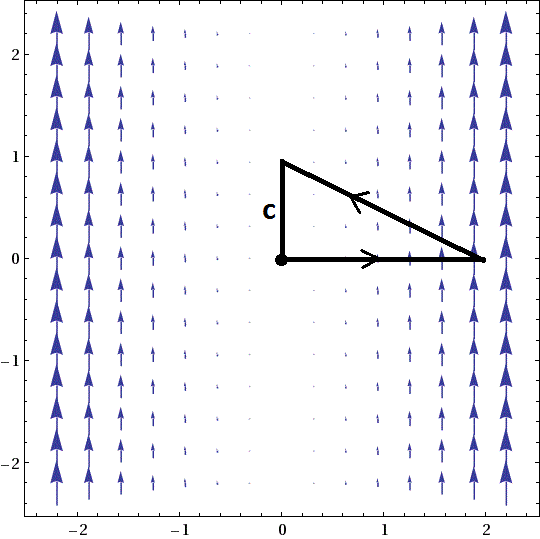
The line integral is zero on the horizontal and vertical sides of the triangle; only on the diagonal is there a non-zero dot product of the field with the tangent vector, with a value about 1⁄2 at the middle and a maximum of about 1 at the right end. Thus, we may guess a total circulation about 1.
To estimate the curl integral, note that for positive x, a paddlewheel would be pushed more strongly counterclockwise by the flow to its right than clockwise by the weaker flow to its left. Thus, curl F is clearly positive, and increases from zero for x = 0 to largish at x = 2; the right half of triangle has area 1⁄2, so the above guess of 1 is reasonable for the double integral of curl F over the triangle.1c. curl F(x,y) = 2x, and D = {(x,y) s.t. 0 ≤ x ≤ 2 , 0 ≤ y ≤ 1−½x}. The double integral is:
∬D curl F dy dx = ∫02 ∫01−½x 2x dy dx = ∫02 2xy |y=01−½x dx = ∫02 2x(1−½x) dx = 4⁄3 , in line with our guess.
1d. We have D = {(x,y) s.t. 0 ≤ y ≤ 1 , 0 ≤ x ≤ 2−2y}, and:
∬D curl F dx dy = ∫01 ∫02−2y 2x dx dy = ∫01 x2 |x=02−2y dy = ∫01 (2−2y)2 dy = 4⁄3 . Any double integral can be done either way (dy dx or dx dy), whichever is more convenient.
1e. The boundary c has three segments: c1(t) = (2t,0) ; c2(t) = (2,0) + [(0,1)−(2,0)]t = (2−2t, t) ; c3(t) = (0, 1−t), where all the parameter ranges are 0 ≤ t ≤ 1. The total circulation is:
∮ F(c) dc = ∮ F(c1) dc1 + ∮ F(c2) dc2 + ∮ F(c3) dc3
= ∫01 F(2t,0) • (2,0) dt + ∫01 F(2−2t, t) • (−2, 1) dt + ∫01 F(0, 1−t) • (0, −1) dt
= ∫01 0 dt + ∫01 (2−2t)2 dt + ∫01 0 dt = 4⁄3 .Behold the Curl Theorem!
2a. The first coordinate is ∂⁄∂x(fg) = ∂f⁄∂x g + f ∂g⁄∂x. Here we may use the one-variable Product Rule since taking the partial derivative ∂⁄∂x is defined as taking the ordinary derivative d⁄dx, while holding y constant. Similarly for the other coordinate. Thus we get the x- and y-coordinates on the left and right sides of the gradient Product Formula.
2b. p(a+h) = b(a+h) • c(a+h) ≈ (b(a) + b'(a)h) • (c(a) + c'(a)h) = b(a)•c(a) + b'(a)•c(a) h + b(a)•c'(a) h + b'(a)•c'(a) h2. The final h2 term is irrelevant for a linear approximation. The coefficient of h gives the derivative p'(a) = b'(a)•c(a) + b(a)•c'(a)
2c. Take the derivative of both sides of c(t)•c(t) = r, obtaining 2 c(t)•c'(t) = 0, meaning the radius vector c(t) and the tangent vector c'(t) are perpendicular (orthogonal).
4a. Solving u = y−x , v = y+x, we get x = −1⁄2u+1⁄2v , y = 1⁄2u+1⁄2v . That is, the inverse of (u,v) = G(x,y) = (y−x, y+x) is:
(x,y) = F(u,v) = (−1⁄2u+1⁄2v , 1⁄2u+1⁄2v). 4b. The columns of the matrix of G(x,y) are G(1,0), G(0,1), having determinant −2. The matrix of F(x,y) can be obtained from the formula above, or from the inverse-matrix formula:[G] = −1 1 1 1 [F] = −1⁄2 1⁄2 1⁄2 1⁄2 . 4c. The parameter domain D* is a triangle with vertices G(0,0) = (0,0), G(1,0) = (−1, 1), G(0,1) = (1,1). This is v-simple:
D* = {(u,v) | 0 ≤ v ≤ 1 , −u ≤ v ≤ u}. 4d. The integral simplifies very nicely upon substitution:∬D exp (y−x)⁄(y+x) dx dy = ∬D* eu/v |det[DF(u,v)]| du dv Note that the stretching factor is the absolute value of the determinant det[DF(u,v)] = det[F] = −1⁄2 .
= ∫1v=0 ∫ u=−v v eu/v 1⁄2 du dv = 1⁄2 ∫1v=0 [v eu/v]u=−vu=v dv
= 1⁄2 ∫1v=0 v (e−e−1) dv = (e−e−1)⁄4 .
In this case, the integrand function became simpler upon substition, and the region D became the mildly more complicated D*. Finally, a fortunate cancellation enabled an explicit solution, which is quite rare.5a. The area of the region is about 3⁄4 the area of the 80×40 rectangle, with an average density of about 3, since the minimum density is near 0 in a small region near the center and about 4 on a large region near the rim. Estimated mass: about 7000g.
5b. The region is an ellipse centered on the orgin, with horzontal radius (semi-major axis) 40cm and vertical radius (semi-minor axis) 20cm. Use the elliptical coordinates F(u,v) = (40u cos(v), 20u sin(v)), with parameter region (u,v) ∈ D* = [0,1] × [0,2π], with stetching factor det[DF(u,v)] = 800u.
5c. Note that f(x(u,v), y(u,v)) = 4u2, so the substitution formula gives: ∬D f(x,y) dx dy = ∫02π∫01 4u2 800u du dv = 1600π ≈ 5027. Pretty close to our estimate.
6a. From the graph, we see that the maximum of f(x,y) is attained either at the local maximum point near (x,y) = (−1,0) or on the boundary at (2,0), and there are two minimum points on the boundary near (1, ±√3). There is also a saddle point near (1,0).
6b. Imagine trimming the contour plot down to the radius 2 boundary disk. Then we again see the local maximum point at (−1,0), and the boundary maximum at (2,0). We again see the boundary minimum points near (1,±√3), where the boundary circle cuts deepest into the dark-colored regions, and there also seems to be a local boundary minimum at (−2,0). The critical points on the boundary are precisely where the boundary curve is tangent to a level curve.
6c. Plotting the gradient vector field, we again see the local maximum with arrows pointing toward it.
Imagining the boundary circle c(t) of radius 2, the critical points are where the gradient ∇f(c(t)) is perpendicular to the direction of c(t). Proof: By the Chain Rule, the critical points of g(t) = f(c(t)) are where 0 = g'(t) = ∇(t) • c'(t).
Now we see that the boundary minumum points on the boundary are a bit to the left of x = 1.7. The orthogonal decomposition of v into p parallel to a and q orthogonal to a is given by p = (v•a)⁄(a•a) a and q = v − p. The reflection along a is thus the linear mapping L(v) = L(p+q) = −p + q = v − 2(v•a)⁄(a•a) a.
Taking a = (a,b) with |a|2 = a2 + b2 = 1, the matrix of L consists of column vectors L(i) = (1−2a2, −2ab) = (b2−a2, −2ab), and L(j) = (−2ab, 1−2b2) = (−2ab, a2−b2), giving the reflection matrix:
where c = b2−a2 and d = −2ab, with c2+d2 = (a2+b2)2 = 1.b2−a2 −2ab −2ab a2−b2 = c d d −c ,
We also have the rotation matrix:a −b b a
To take compositions of these mappings, we multiply their matrices. Inspecting the result shows that multiplying two different reflection matrices gives a rotation matrix, and multiplying a reflection times a rotation gives a new reflection. (Also, multiplying two rotations gives a rotation.) These formulas are all intimately related to the angle addition formulas for sin and cos.
- 10/21 Midterm Exam
- 10/23 Lect 23. ⊞ Vectors in R3 and Rn. Determinants.
⊞ Solutions- Vector x = (x1, . . . , xn) ∈ Rn
- Dot product
u•v =
(u1, . . . ,un)•(v1, . . . , vn)
= u1v1 + ··· + unvn
Geometrically: u•v = |u| |v| cos θuv - Linear subspace V ⊂ Rn or R3,
k-dimensional with basis {v1, . . . , vk}
Parametrize: V = { v = L(t1, . . . , tk) | t1, . . . , tk ∈ R },
for linear function L : Rk → Rn, L(t1, . . . , tk) = t1v1 + ··· + tkvk
Equations: V = { v ∈ Rn | q1•v = ··· = qn−k•v = 0 }
for orthogonal vectors q1, . . . , qn−k ⊥ V - Affine subspace A = V + a ⊂ Rn or R3 for constant vector a
Parametrize by function P(t1, . . . , tk) = L(t1, . . . , tk) + a
Equations: A = { v ∈ Rn | q1•(v−a) = ··· = qn−k•(v−a) = 0 } - Determinant det(u,v,w) = signed volume of parallelopiped with edges from the origin parallel to u,v,w.
Sign is positive (+) if u,v,w form a right-handed coordinate system
negative (−) if they form a left-handed one. - Properties: det(u,v,w)
= −det(v,u,w)
= −det(u,w,v)
det(su+s'u',v,w) = s det(u,v,w) + s' det(u',v,w), similarly for variables v, w
det(i,j,k) = 1; also det(i,i,j) = 0, etc. - Formula for determinant:
det u1 u2 u3 v1 v2 v3 w1 w2 w3 = u1v2w3 − u1v3w2 − u2v1w3 + u2v3w1 + u3v1w2 − u3v2w1 = ∑σ sgn(σ) uσ(1)vσ(2)wσ(3) ,
We can denote a permutation by listing σ(1)σ(2)σ(3). For example, σ(1) = 3, σ(2) = 2, σ(3) = 1 is denoted σ = 321 - The sign of a permutation sgn(σ) equals +1 if σ is obtained from the identity permutation ε(i) = i by switching an even number of pairs of outputs; and sgn(σ) equals −1 if it is obtained by switching an odd number of pairs of outputs.
For example the permutation σ = 321 is obtained from ε = 123 by switching the single pair of outputs 1 and 3, so sgn(σ) = −1; or switch 12, then 23, then 12, again sgn(σ) = −1.
HW: Extra Credit HW due Thu 10/31.- Consider the affine plane A ⊂ R3 containing the points
a = (0,1,1), b = (1,1,2), c = (1,2,0). (As usual, when we define a point by a vector,
we mean the endpoint of the vector starting at the origin.)
- Find two vectors parallel to the plane, for example from a to b, and from a to c.
- Write a parametric formula P(t1,t2) = (x(t1,t2), y(t1,t2), z(t1,t2)) which outputs the points of the plane as s,t vary. Hint: Start at a and move along the two directions from part (a).
- Find an orthogonal vector q with q•(v−a) = 0 for v ∈ A. Write a defining linear equation satisfied by all v = (x,y,z) ∈ A, in the form ax + by + cz = d.
- Determine the distance from the point r = (3,4,5) to the plane. Hint: The distance is the difference in height with respect to the unit orthogonal vector q⁄|q|.
- Consider the affine line C ⊂ R3 through the points a = (0,1,1) and b = (1,1,2) from #1.
- Find a parametric form c(t) = (x(t),y(t),z(t)) for C.
- Find two vectors q1, q2 which are orthogonal to the direction of C. Write two defining equations satisfied by all v = (x,y,z) ∈ C.
- For each ordered triple of vectors u, v, w:
- Sketch the vectors and the parallelopiped they span.
- Determine whether they form a right-handed triple: that is can you point your right index finger along u, middle finger along v, thumb along w,
so that the thumb is not bent behind or through
the plane of the other two fingers.
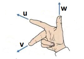
- Determine the signed volume of the parallelopiped by evaluating the determinant det(u; v; w). Verify that a right-handed triple has positive det, a left-handed one has negative det.
- u = (1,1,0), v = (1,0,1), w = (1,1,2)
- u = (1,0,1), v = (1,1,0), w = (1,1,2)
- u = (1,1,0), v = (1,0,1), w = (2,1,1)
1a. Directions along A: v1 = b−a = (1,0,1) , v2 = c−a = (1,1,−1).
1b. P(t1,t2) = t1v1 + t2v2 + a = (t1+t2, 1+t2, 1+t1−t2).
1c. The number of independent orthogonal vectors is n−k = 3−2 = 1. We want q = (q1,q2,q3) with q•v1 = 0 and q•v2 = 0, giving the linear system:
q1 + q3 = 0 , q1 + q2 − q3 = 0. Solving this by elimination gives q2 = −2 q1 and q3 = −q1, or q = q1(1,−2,−1) for any q1 ∈ R. Taking q1 = 1 gives a specific normal vector q = (1,−2,−1) .Thus, a defining equation is q•(v−a) = 0, which in coordinates v = (x,y,z) can be simplified to:
x − 2y − z = − 3 We can check that the original points a, b, c all satisfy this equation.1d. Let r − a = (3,3,4) be the vector from the basepoint a = (0,1,1) on V to the point r = (3,4,5) off of V. The orthogonal distance from V to r can be obtained by projecting r − a on the orthogonal vector q; or simply by dotting r − a with the unit vector q⁄|q|:
(r−a) • q⁄|q| = 7⁄√6. 2. The affine line has direction vector v1 = b−a = (1,0,1), parametrized by c(t) = tv1 + a = (t,1,t+1).
There are n−k = 3−1 = 2 independent orthogonal vectors satisfying q•v1 = 0, i.e. q = (q1, q2, −q1) = q1(1,0,−1) + q2(0,1,0), giving q1 = (1,0,−1) and q2 = (0,1,0). The curve C is the set of points v = (x,y,z) satisfying the two equations qi•(v−a), i.e.: x − z = −1 , y = 1.3a. The triple u = (1,1,0), v = (1,0,1), w = (1,1,2):
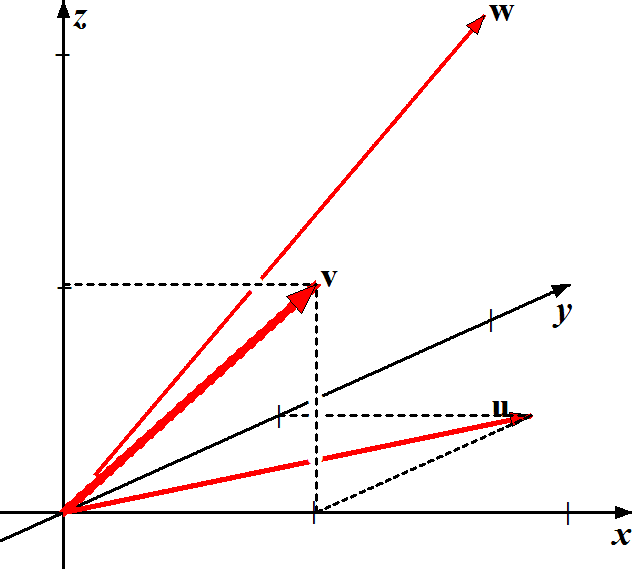
Notice that we draw the x,y,z axes as a right-handed triple, and v is in the xz-plane in the foreground, whereas w recedes into the picture. This is a left-handed system: model it with your left palm up, index finger horizontal along u, middle finger almost vertical along v, thumb pointing away from you along w. The left-handedness is reflected in the determinant −2, the signed volume of the corresponding parallelopiped, as we will see next time.
We compute the determinant, the signed volume of the parallelepiped spanned by the three vectors, writing u, v, w as the columns of a 3×3 matrix, with one term for each permutation of {1,2,3}:
det(u, v, w) = det 1 1 0 1 0 1 1 1 2 = u1v2w3 − u1v3w2 − u2v1w3 + u2v3w1 + u3v1w2 − u3v2w1 = 1·0·2 − 1·1·1 − 1·1·2 + 1·1·1 + 0·1·1 − 0·1·1 = −2.
det(u,v,w) = u1 det(v(1); w(1)) − u2 det(v(2); w(2)) + u3 det(v(3); w(3)) = 1 det(0,1 | 1,2) − 1 det(1,1 | 1,2) + 0 det(1,0 | 1,1) = −1 − 1 + 0 = −2.
The negative value verifies the left-handedness.
3b. The triple u = (1,0,1), v = (1,1,0), w = (1,1,2), with the first two vectors switched from part (a), is right-handed, with the opposite determinant: det(u,v,w) = 2.
3c. The triple u = (1,1,0), v = (1,0,1), w = (2,1,1) has w = u + v, which means the three vectors all lie in the same plane: they are linearly dependent. Thus, the parallelepiped is flat, with volume zero, and we may verify det(u,v,w) = 0. The triple is degenerate, neither right- nor left-handed.
- 10/24 Recitation 9.
- 10/25 Lect 24. ⊞ Cross product
⊞ Solutions- Linear function ℓ: R3 → R
ℓ(x,y,z) = ax+by+cz = (a,b,c)•(x,y,z), ℓ(v) = q•v for q = (a,b,c) Picture ℓ(v) as height of v in direction q, scaled by |q|
Height ℓ(v) = 0 defines plane orthogonal to q, through origin
Other level surfaces ℓ(v) = c define affine planes orthogonal to q
Actual height = (length of projection of v onto direction q) = q⁄|q| • v - Cross product on vectors in R3 only (not Rn),
giving vec × vec = vec
Geometrically: u×v = q, the vector which produces the lin fun ℓ(w) = det(u,v,w) = q•w
Given u, v, the cross product u×v is the unique vector such that for all w.:det(u,v,w) = (u×v) • w . - Formula for u×v
ℓ(x,y,z) = det u1 u2 u3 v1 v2 v3 x y z = u1v2z − u1v3y − u2v1z + u2v3x + u3v1y − u3v2x = (u2v3− u3v2) x + (−u1v3+u3v1) y + (u1v2− u2v1) z = q • (x,y,z) q = u×v = (u1,u2,u3) × (v1,v2,v3) = (u2v3− u3v2 , −u1v3+u3v1 , u1v2− u2v1)
- Determinant cofactor expansion
u × v = det u1 u2 u3 v1 v2 v3 i j k = det u2 u3 v2 v3 i − det u1 u3 v1 v3 j + det u1 u2 v1 v2 k - Properties of u×v come from
properties of det
u×v orthogonal to both u,v: (u×v)•u = (u×v)•v = 0
u, v, u×v form a right-handed basis
anti-commutative: u×v = −v×u, u×u = 0
distributive: (u+u') × v = u×v + u'×v
linear: (au)×v = u×(av) = a u×v - Length |u×v| = area of parallelogram spanned by u,v in R3
= |u| |v| sin(θuv)
Proof: Geometrically, volume(u,v,w) = (base area of u,v parallelogram) (height of w perp to u & v).
Algebraically, volume(u,v,w) = det(u,v,w) = (u×v)•w = |u×v| u×v⁄|u×v|•w
= |u×v| (height of w along direction q). Cancelling (height of w), we get area(u,v) = |u×v|.
Extra Credit HW due Thu 10/31.
HW:- Recall from the previous HW the affine plane A
containing the points a = (0,1,1), b = (1,1,2),
c = (1,2,0).
- Re-compute the vector q orthogonal to A as the cross product: q = (b−a)×(c−a)
- For a general point w = (x,y,z) ∈ A, expand the vector equation q•(w−a) = 0, or equivalently q•w = q•a, to again get the explicit coordinate equation ax + by + cz = d defining A.
- Also recall the vectors u = (1,1,0), v = (1,0,1),
w = (1,1,2).
- Compute the cross product q = u×v.
- Compute the volume of the u, v, w parallelopiped by evaluating the triple product (u×v)•w = q•w = det(u,v,w).
- The cross product u×v
can only be defined for three dimensional vectors,
but determinant exists in any dimension Rn,
and the formula
det(u1, . . . , un−1, w) = ℓ(w) = q • w for all w defines a unique vector q, which we may think of as a "product" of n−1 vectors: q = u1×···×un−1 .- For n = 2, this operation acts on a single vector u, giving u×. What familiar operation is this?
- Find a cofactor expansion formula for the cross product of 3 vectors in R4.
1a. The directions parallel to the plane are u = b − a = (1,0,1) and v = c − a = (1,1,−1), giving the orthogonal direction q = u × v = (−1,2,1).
1b. The equation q • w = q • a becomes (−1,2,1) • (x,y,z) = (−1,2,1) • (0,1,1), or −x + 2y + z = 3. This agrees with the previous HW.
2a. q = (1,1,0) × (1,0,1) = (1,−1,−1)
2b. q • w = (1,−1,−1) • (1,1,2) = −2. This agrees with the previous HW.
3a. The determinant formula defining q = u× is: det(u, w) = q • w. Writing u = (u1, u2), w = (x,y), and q = (a,b), this becomes u1y − u2x = ax + by, so q = (−u2, u1), which is the counterclockwise perpendicular vector to (u1, u2). That is, u× = u⊥.
3b. For three vectors u, v, w ∈ R4, their cross product q = u×v×w is the vector orthogonal to all three and with length equal to the volume of the three-dimensional box spanned by them. Its coordinates are the coefficients of x1, . . . , x4 in the determinant:
These can be found using the cofactor expansion along the last column, in which the coefficient of each xi is given by the determinant of the complementary 3×3 submatrix (with alternating ± signs).det u1 u2 u3 u4 v1 v2 v3 v4 w1 w2 w3 w4 x1 x2 x3 x4 .
- 10/28 Lect 25. ⊞ Linear Functions on R3
⊞ Solutions- c : R → R3, c(t) = tu parametrized line
- L : R2 → R3, L(t,s) = tu + sv parametrized plane
- ℓ : R3 → R, ℓ(x) = q•x height of x in dir q, scaled so that ℓ(q) = |q|2
- P : R3 → R2,
Ker(P) = Rq with P(q) = 0, orthogonal plane V = q⊥,
P projects (collapses) R3 along q to V ≅ R2 - L : R3 → R3,
linear transformation, motion of space around origin, possibly with stretching or distortion
Examples: rotation around an axis, reflection Reflq(x) = x − 2(x•q⁄q•q) q
HW:- Use the determinant definition of cross product to prove the following properties
- Any triple u, v, u×v is a right-handed basis (if u,v ≠ 0 and u ≠ c v)
- u×u = 0
- i×j = k, j×k = i, k×i = j
- Find the 3×3 matrix of each of the following linear transformations of R3
- Orthogonal reflection across the plane V perpendicular to q = (1,2,3)
- Rotation by 90° around the x-axis
- Rotation by 90° around the y-axis
- The composition of the previous two rotations. Describe the resulting motion geometrically.
- The shear transformation which takes i,j,k to the vectors i, i+j, i+j+k. Does this transformation distort volume?
1a. The triple u, v, u×v is a right-handed basis exactly if its determinant is positive. We check:det(u, v, u×v) = (u×v)•(u×v) = |u×v|2 ≥ 0 This can only fail to be positive if |u×v| = |u| |v| sin θuv = 0, i.e. if θ = 0° or 180° and u = c v; and if u or v = 0.1b. We have: (u×u)•w = det(u, u, w) = 0, by the vanishing properties of det.
1c. These follow directly from the determinant formula for i×j, etc.
2a. We know L = Refq(v) = v − 2(v•q⁄q•q) q for q = (1,2,3). Its matrix is:
[L] = [L(i) | L(j) | L(k)] = 1⁄14 12 −4 −6 −4 6 −12 −6 −12 −4 . 2b. The mapping R1 = Rot90,i is 90° around the x-axis. (Here we use a right-hand rule, so that if we point the thumb along the x-axis, the yz-plane is rotated in the direction of the fingers.) The matrix is:
[R1] = [R1(i) | R1(j) | R1(k)] = 1⁄14 1 0 0 0 0 1 0 −1 0 . 2d. The matrix of R3(x) = R2(R1(x)) is gotten by matrix multiplication: [R3] = [R2]•[R1]. The composition of any two rotations is again a rotation.
2e. The shear rotation has a matrix [S] with det[S] = 1, so it does preserve volume, even though it distorts angles.
- 10/30 Lect 26. ⊞ Functions f : R3 → R.
⊞ Soln- f(x,y,z) can represent temperature, pressure, potential energy, etc.;
or measure some geometric property of v = (x,y,z), such as radius or height - Picture f using level surfaces f(x,y,z) = const;
surface through a is f(x,y,z) = f(a)
like onion or pastry layers slicing up the space R3 - Gradient vector field ∇f
= (∂f⁄∂x,
∂f⁄∂y,
∂f⁄∂z)
direction of fastest increase of f, length = max rate of increase - Gradient ∇f(a) is
perpendicular to level surface through a
dir of max increase ⊥ directions of no increase - Ex: linear ℓ(v) = q•v,
ℓ(x,y,z) = ax+by+cz
measures scaled height in direction q
level surfaces are parallel planes - Ex: f(v) = |v|2, f(x,y,z) = x2+y2+z2 measures
radius
level surfaces are concentric spheres - Ex: f(x,y,z) = x2+y2−z2
level surface f = 0 is circular cone around z-axis
f = c is hyperboloid of one sheet (c > 0) or two sheets (c < 0)
HW:- Consider the function f(x,y,z) = xy−z2.
- For each level surface f(x,y,z) = 0, 1, −1, write the surface as one or more graphs of functions z = g(x,y), and sketch the surface. Describe a general level surface f(x,y,z) = c. (If you have trouble visualizing, use Wolfram Alpha.)
- Find the gradient ∇f(a) at a = (1,2,3). Write an equation for the tangent plane to the surface at a.
- Consider the surface defined by a graph z = g(x,y).
- Write this as a level surface f(x,y,z) = const. What do the other level surfaces of f(x,y,z) look like?
- Write the tangent plane of the surface at a point (a,b,c) = (a,b,g(a,b)) in terms of the partial derivatives of g. Compare this equation to the tangent plane perpendicular to the gradient ∇f(a,b,c).
1a. The level surface f(x,y,z) = xy−z2 = 0 is a circular cone around the axis (1,−1,0). Its other level surfaces are hyperboloids of one or two sheets:
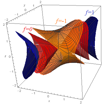
1b. We have ∇f(x,y,z) = (∂⁄∂x, ∂⁄∂y, ∂⁄∂z)(xy−z2) = (y, x, −2z), so ∇f(a) = ∇f(1,2,3) = (2,1,−6).
The level surface through a = (1,2,3) is f(x,y,z) = f(1,2,3) = −7, and the tangent plane to this surface is orthogonal to the gradient vector at a. The tangent plane equation is ∇f(a)•(v−a) = 0, i.e.(2, 1, −6)•(x−1, y−2, z−3) = 2(x−1) + (y−2) − 6(z−3) = 0,
2a. The function f(x,y,z) = g(x,y) − z has the level surface f(x,y,z) = 0 equal to the graph z = g(x,y). Any other level surface f = k is the graph z = g(x,y) + k, an up or down translate of z = g(x,y).
2b. The tangent plane of z = g(x,y) at the point (a,b,g(a,b)) is the graph of the linear approximation:
z = g(a,b) + ∂g⁄∂x(a,b) (x−a) + ∂g⁄∂y(a,b) (y−b). Alternatively, the tangent plane is orthogonal to the gradient ∇f(x,y,z) = (∂g⁄∂x, ∂g⁄∂y, −1) at (x,y,z) = (a,b,g(a,b)):(∂g⁄∂x(a,b), ∂g⁄∂y(a,b), −1)•(x−a, y−b, z−g(a,b)) = ∂g⁄∂x(a,b) (x−a) + ∂g⁄∂y(a,b) (y−b) − (z−g(a,b)) = 0, which reduces to the previous equation.- 10/31 Recitation 10. Curves & surfaces in space, Frenet frame.
- 11/1 Lect 27. ⊞ Cylind & spherical coords, param surfaces
⊞ Soln- Cylindrical coords: Cyl(r,θ,z) =
(r cos(θ), r sin(θ), z)
r = radius from z-axis, θ = turn from xz-plane, z = height - Spherical coords: Sph(ρ,θ,φ)
= (ρ sin(φ) cos(θ),
ρ sin(φ) sin(θ),
ρ cos(φ))
ρ = radius from origin, θ = turn from xz-plane, φ = tilt from z-axis
z = ρ cos(φ), r = ρ sin(φ),
x = r cos(θ) = ρ sin(φ) cos(θ), y = r sin(θ) = ρ sin(φ) sin(θ) - Toroidal coords:
Tor(r,θ,φ) = ((R+r cos(φ))cos(θ),
(R+r cos(φ))sin(θ), r sin(φ))
Decompose v = (x,y,z) = Ru + rw with |u| = |w| = 1
R = fixed radius of core ring, Ru = (R cos(θ), R sin(θ), 0)
w points from core point Ru to v on sectional circle of radius r
φ = tilt of w from xy-plane, w = r cos(φ)u + r sin(φ)k - Frenet frame ([MT] 4.2, Ex 16, 20, p. 235):
curve c(t) = (x(t), y(t), z(t))
u(t) = c'(t)⁄|c'(t)|, unit tangent vector; n(t) = u'(t)⁄|u'(t)|, unit normal vector (normal acceleration)
b(t) = u(t) × n(t), binormal vector
{u(t), n(t), b(t)} forms orthonormal basis of R3 at each point c(t) - Change of variables for parametrized solid region D.
Parametrization F(u,v,w) = (x(u,v,w), y(u,v,w), z(u,v,w)) for (u,v,w) ∈ D* parameter region.
Integral of f(x,y,z) over region:
∫∫∫D f(x,y,z) dx dy dz = ∫∫∫D* f(x(u,v,w), y(u,v,w), z(u,v,w)) det[DF(u,v,w)] du dv dw - Pappus Centroid Theorem: Vol of solid of revolution = area × distance traveled by center of gravity
HW: Start WHW 9 due 11/7 below.- Parametrizing the torus with core circle radius 2,
thickness radius 1.
- Compute the Frenet frame u(t), n(t),
b(t) for the core circle
c(t) = (2 cos(t), 2 sin(t), 0),
simplifying with trig identities.
Write out the Frenet coordinate parametrization:
F(t,p,q) = c(t) + p n(t) + q b(t) = (x(t,p,q), y(t,p,q), z(t,p,q)). - Write out the toroidal coordinate map by converting the Frenet frame to polar coordinates (r,φ) in the n(t) & b(t) plane at each point of the core circle. That is, T(θ, r, φ) is at angle θ ∈ [0,2π] of the core circle, radius r ≥ 0 from the core circle, and tilt φ ∈ [0,2π] from the horizontal plane.
- Use the above function to draw a parametrized torus surface T(θ, 1, φ) on Mathematica (install for free) or Wolfram Alpha.
- Compute the Frenet frame u(t), n(t),
b(t) for the core circle
c(t) = (2 cos(t), 2 sin(t), 0),
simplifying with trig identities.
Write out the Frenet coordinate parametrization:
- Determine the inverse function of the spherical coordinate map Sph. That is, write ρ, θ, φ as functions of x,y,z.
- Sphere D of radius R has volume 4⁄3 π R3.
- Verify the spherical coordinate stretching factor
det[Sph(r,θ,φ)] = −ρ2 sin(φ).
Use the cofactor expansion of a determinant:det x y z u1 u2 u3 v1 v2 v3 = det u1 u2 u3 v1 v2 v3 x y z = det u2 u3 v2 v3 x − det u1 u3 v1 v3 y + det u1 u2 v1 v2 z. - Compute the volume of sphere D by a spherical substitution D = Sph(D*), where D* is a rectangular parameter domain in (ρ,θ,φ) space: Vol(D) = ∫∫∫D* ρ2 sin(φ) dφ dθ dρ.
- Try to determine this volume in rectangular coordinates,
Vol(D) = ∫∫∫D 1 dz dy dx,
writing the sphere as the set of (x,y,z) with:
−R ≤ x ≤ R
−√(R2−x2) ≤ y ≤ √(R2−x2)
−√(R2−x2−y2) ≤ z ≤ √(R2−x2−z2).
- Verify the spherical coordinate stretching factor
det[Sph(r,θ,φ)] = −ρ2 sin(φ).
- For the region under a graph curve z = g(x) in the xz-plane and above the interval x ∈ [0,R], parametrize its solid of revolution around the z-axis, and compute its volume using cylindrical coordinates (r,θ,z). Which Calc I method does this correspond to?
- Extra Credit: Prove Pappus' Centroid Theorem:
The volume of a solid of revolution of a region
is equal to the area of the region, times the distance traveled by its center of gravity.
The center of gravity cent(D) of a plane region D
is the average position of a point of D.
To compute cent(D) = (x, y), take the average of each coordinate function over D:
x = 1⁄area(D) ∫∫∫D x dx dy and similarly for y. Now assume D is rotated around the x-axis. How far is cent(D) rotated?
Also, the theorem can be generalized to moving D along the Frenet frame of any curve, not just a circle . . . .
1a. For the circle c(t) = (2 cos(t), 2 sin(t), 0), we have the tangent vector c'(t) = 2(−sin(t), cos(t), 0) and the unit tangent vector is:u(t) = (−sin(t), cos(t), 0). Then the normal (centripetal) acceleration is u'(t) = −(cos(t), sin(t), 0), which has unit length, so it is equal to the unit normal acceleration:n(t) = −(cos(t), sin(t), 0). Finally, the binormal is:b(t) = u(t) × n(t) = (0,0,1). These define the Frenet frame u(t), n(t), b(t), an orthonormal basis of space defined for each point c(t), which we can use just like i, j, k.The Frenet coordinates of c(t) are thus:
F(t,p,q) = (2 cos(t) − p cos(t), 2 sin(t) − p sin(t), q) 1b. We trace a circle of radius r around each point c(t), in the plane with basis n(t), b(t):P(t,φ) = c(t) + r cos(φ) n(t) + r sin(φ) b(t) Taking r = 1 gives the torus with thickness radius 1.
= (2 cos(t) − r cos(φ) cos(t), 2 sin(t) − r cos(φ) sin(t), r sin(φ))1c. Wolfram gives:
Here is a Mathematica file you can use to learn relevant commands
2. Given (x,y,z), the radius from the z-axis is r = √(x2+y2), and the radius from the origin is the hypotenuse of the right triangle with vertices (0,0,0), (x,y,0), (x,y,z):
ρ = √(r2+z2) = √(x2+y2+z2). The turn of (x,y,z) from the xz-plane is the same as the turn of (x,y,0) from the x-axis:θ = arccos(x⁄√(x2+y2)) = arcsin(y⁄√(x2+y2)) = arctan(y⁄x). The tilt of (x,y,z) from the z-axis is φ, satisfying z = ρ cos(φ) and r = ρ sin(φ), so thatφ = arccos(z⁄√(x2+y2+z2)) = arcsin(√(x2+y2)⁄√(x2+y2+z2)) = arctan(√(x2+y2)⁄z). Therefore:
(ρ,θ,φ) = Sph−1(x,y,z) = (√(x2+y2+z2, arccos(x⁄√(x2+y2)), arccos(z⁄√(x2+y2+z2)) ), assuming 0 ≤ arccos(t) ≤ π and y ≥ 0, 0 ≤ θ ≤ π. For general y, we should replace the above θ by sgn(y) θ, where sgn(y) = +1 for y ≥ 0 and sgn(y) = −1 for y < 0.3a. Taking 2×2 subdeterminants of the Jacobian DS(ρ,θ,φ) of S = Sph gives the cross product:
∂S⁄∂θ × ∂S⁄∂φ = −ρ2 sin(φ) (cos(θ)sin(φ), sin(θ)sin(φ), cos(φ)), and taking the dot product with ∂S⁄∂ρ gives the Jacobian determinant:det[DS] = ∂S⁄∂ρ • (∂S⁄∂θ × ∂S⁄∂φ) 3b. Since the integrand factors into functions of the individual variables, and the rectangular parameter domain is D* a Cartesian product of intervals (ρ,θ,φ) ∈ [0,R]×[0,2π]×[0,π], the triple integral factors into a product of single-variable integrals:
= −ρ2 sin(φ) ( cos2(θ)sin2(φ) + sin2(θ)sin2(φ) + cos2(φ) ) = −ρ2 sin(φ).Vol(D) = ∫Rr=0 ∫2πθ=0 ∫2πφ=0 ρ2 sin(φ) dφ dθ dρ 3c. Taking advantage of symmetry, we can reduce to the positive side of each integral:
= (∫Rr=0 ρ2 dρ) (∫2πθ=0 dθ) (∫πφ=0 sin(φ) dφ) . = (1⁄3R3) (2π) (2).Vol(D) = 8 ∫x=0R∫y=0√(R2−x2)∫z=0√(R2−x2−y2) dz dy dx Here we used the antiderivative
= 8 ∫x=0R∫y=0√(R2−x2) √(R2−x2−y2) dy dx
= 4 ∫x=0R [ y√(R2−x2−y2) + (R2−x2) arctan(y⁄√(R2−x2−y2)) ]y=0√(R2−x2) dx
= 4 ∫x=0R (R2−x2) π⁄2 dx = 2π(R3 − R3⁄3).∫ √(a2−y2) dy = 1⁄2[ y√(a2−y2) + a2 arctan(y⁄√(a2−y2)) ], and thatarctan(√(R2−x2)⁄0+) = limu→∞ arctan(u) = π⁄2 . 4. The solid of revolution D is parametrized by the (r,θ,z) parameter region D* with 0 ≤ r ≤ R, 0 ≤ θ ≤ 2π, 0 ≤ z ≤ g(r). The stretching factor of the cylindrical parametrization Cyl(r,θ,z) = (r cos(θ), r sin(θ), z) is the same as for polar coordinates, namely r, so the volume is:Vol(D) = ∫r=0R∫θ=02π∫z=0g(r) r dz dθ dr This is the "shell method" volume formula for a solid of revolution.
= (∫θ=02π dθ) (∫r=0R r g(r) dr) = ∫r=0R 2πr g(r) dr.
- 11/4 Lect 28. ⊞ Area of parametric surface.
⊞ Solutions- Parameter region S* ⊂ R2
for surface S ⊂ R3
Parametrization P : S* → S, P(u,v) = (x(u,v), y(u,v), z(u,v)) - Find stretching factor of P(u,v) near a point (u,v) = (uo,vo)
Same as stretching factor of linear approx
DP(uo,vo) = [∂P⁄∂u | ∂P⁄∂v ] Jacobian matrix 3×2
with column vector ∂P⁄∂u = (∂x⁄∂u, ∂y⁄∂u, ∂z⁄∂u), and similar for ∂P⁄∂v
Linear mapping DP(a,b) : R2 → R2 stretches unit square
to parallelogram in R3 spanned by ∂P⁄∂u , ∂P⁄∂v
Area of parallelogram spanned by a, b is length |a×b| = |a||b|sin(θab)
Stretching factor is: |∂P⁄∂u × ∂P⁄∂v| - Area = limit of sum of areas of small parallelograms in S
Area(S) = ∬S* |∂P⁄∂u×∂P⁄∂v| du dv
HW: WHW 9 due 11/7 below.- Consider the sadddle surface given by the graph z = x2 − y2 above the unit square
(x,y) ∈ [0,1] × [0,1]; that is
0 ≤ x ≤ 1 and 0 ≤ y ≤ 1.
- Find a parametrization P : S* → S. Hint: What parameter variables control the position of a point on S?
- Find the Jacobian matrix dP(u,v), and the stretching factor |∂P⁄∂u×∂P⁄∂v|.
- Set up a double integral to evaluate the area. Use Wolfram Alpha to find numerical approximation.
- Find the lengths of the edge curves of S, above the x- and y-axes. (Parametrize the curves and compute the length L = ∮ |dc|.) How does the area compare to the product of the edge-lengths, and to the area of the parameter region S*?
- Write and simplify the area integrals for
- A general graph z = g(x,y) for (x,y) in a plane region D ∈ R2
- A general surface of revolution, rotating a curve y = f(x), for x ∈ [a,b], around the x-axis. (Assume f(x) ≥ 0.)
- Check your answer in (b) by applying it to the section of a right circular cone with height a and base radius b: this surface has equation z = a⁄b √(x2+y2). We can unroll the surface to get a circular sector with radius √(a2+b2) and outer circumference 2πb, and we can find its area without calculus.
- Compute the following integrals
- The sphere of radius r. Hint: The vector ∂P⁄∂u×∂P⁄∂v for a spherical parametrization P(θ, φ) was computed in the previous HW solutions, as a step in computing det[DSph(ρ, θ, φ)]. In fact, the volume and area stretching factors are the same, since dρ is not stretched by the Sph mapping.
- Compute the surface area and the enclosed volume of the torus with core radius R, sectional radius r (see previous lecture). Hint: Again, the volume and area stretching factors will be the same, since dr is not stretched by the toroidal coordinate mapping (see previous lecture).
- Review of cross product. Let a = (1,2,−1),
b = (1,0,1).
- Compute a×b
- Verify the defining property of cross product: det(a,b,v) = (a×b) • v.
- Verify that a×b is orthogonal to a, b.
- Verify that |a×b| = |a| |b| sin(θab), and that this is the area of the parallelogram (actually a rectangle) spanned by a, b. Hint: What is the familiar way to determine cos(θab)?
1. The parametrization P(u,v) = (u, v, u2−v2) gives A = ∫10∫10 √(1+4x2+4x2) dx dy ≈ 1.86 . The edge above the x-axis is c(t) = (0, t, −t2), with length ∫10√(1+4t2) dt ≈ 1.48. The other edge curve has the same length, and their product is 1.492 ≈ 2.19 , bigger than the actual area, which is in turn bigger than 1, the parameter region area.2a. The graph z = f(x,y) is parametrized by T(x,y) = (x, y, f(x,y)), giving stretching factor:
|∂T⁄∂x × ∂T⁄∂y| = |(1, 0, ∂f⁄∂x) × (0, 1, ∂f⁄∂y)|
= |(−∂f⁄∂x ,−∂f⁄∂y , 1)| = √(1 + (∂f⁄∂x)2 + (∂f⁄∂y)2).
The area is:A = ∬ √(1 + (∂f⁄∂x)2 + (∂f⁄∂y)2) dx dy.
This will usually be over some finite region (x,y) ∈ R* in the xy-plane.2b. The surface of revolution z = g(√(x2+y2) is parametrized by the cylindrical coordinate mapping T(r,θ) = (r cos(θ), r sin(θ), g(r)), giving stretching factor:
|∂T⁄∂r × ∂T⁄∂θ| = |(cos(θ), sin(θ), g'(r)) × (−r sin(θ), r cos(θ), 0)|
= |r (cos(θ) g'(r) , sin(θ) g'(r) , 1)| = r √(1 + g'(r)2) .
The area is:A = ∬ r √(1 + g'(r)2) dr dθ
Again, this is over a parameter region (r, θ) ∈ R*.2c. The right circlular cone with height a and base radius b has a vertex-to-rim radius of ρ = √(a2+b2), and a rim circumference C = 2πb. We can unroll the lateral surface into a sector of a circle of radius ρ, with circular arc C. The area A of a sector is proportional to its circular arc, so C⁄2πρ = A⁄πρ2 . That is: A = πb√(a2+b2).
The cone is parametrized by T(r,θ) = (r cos(θ), r sin(θ), a⁄b r) for 0 ≤ r ≤ b and 0 ≤ θ ≤ 2π. The formula of part (b) becomes:
A = ∬ r √(1 + g'(r)2) dr dθ = ∫02π ∫0b r √(1 + (a⁄b)2) dr dθ
= [ 2π√(1 + (a⁄b)2) r2⁄2 ]r=0b = πb√(a2+b2).3a. The sphere of radius ρ = R is parametrized by P(θ,φ) = Sph(R,θ,φ), with
∂P⁄∂θ × ∂P⁄∂φ = −ρ2 sin(φ) (cos(θ)sin(φ), sin(θ)sin(φ), cos(φ)), and area stretching factor|∂P⁄∂θ × ∂P⁄∂φ| = R2 sin(φ). The area is thus:Area = ∫θ=02π∫φ=0π R2 sin(φ) dθ dφ = 4πR2.
3b. Consider the toroidal coordinate mapping:
T(r,θ,φ) = R (cos(θ), sin(θ), 0) + r cos(φ) (cos(θ), sin(θ), 0) + (0, 0, r sin(φ)). The first term parametrizes the core circle of radius R in the xy-plane by the angle θ, similar to the usual polar coordinate mapping. On a vertical circle of radius r, a radial vector tilted by angle φ from horizontal has horizontal component r cos(φ) and vertical component r sin(φ). This horizontal component should be in direction (cos(θ), sin(θ), 0), giving the second term, and the vertical component should be in direction (0, 0, 1), giving the third term.The Jacobian derivative matrix is:
[DT] = cos(φ) cos(θ) cos(φ) sin(θ) sin(φ) −sin(θ)(r cos(φ)+R) cos(θ)(r cos(φ)+R) 0 −r sin(φ) cos(θ) −r sin(φ) sin(θ) r cos(φ) .
The Jacobian determinant simplifies to: det[DT] = r(R + r cos(φ)).
W|A can compute this if you input the above 3×3 matrix in the format {{a,b,c},{d,e,f},{g,h,i}}. The determinant remains the same if you transpose rows and columns.For fixed r, the torus surface parametrization T(θ,φ) = T(r,θ,φ) gives the tangent vectors ∂T⁄∂θ , ∂T⁄∂φ of T(θ,φ) are the same as the corresponding columns of T(r,θ,φ) above. The normal vector is:
n = ∂T⁄∂θ × ∂T⁄∂φ = r (R + r cos(φ)) (cos(φ) cos(θ), cos(φ) sin(θ), sin(φ)).
This is a scalar times the unit vector (cos(φ) cos(θ), cos(φ) sin(θ), sin(φ)), which happens to be the same as ∂T⁄∂r : that is, the radial derivative vector of T is the unit orthogonal to the other two derivative vectors, which is evident from the geometry. Therefore the length of the cross product is the same as the volume stretching factor above: |n| = r (R + r cos(φ)).The area of the torus is thus:
A = ∫02π∫02π r (R + r cos(φ)) dφ dθ
= [2π r (Rφ + r sin(φ))]2πφ=0 = 4π2rR.
We temporarily denote the fixed sectional radius by r0, so that the solid torus has 0 ≤ r ≤ r0. Then the volume is:V = ∫0r0∫02π∫02π r (R + r cos(φ)) dφ dθ dr
= ∫0r0 A(r) dr = ∫0r0 4π2rR dr = 2π2r02R .
Then replacing r0 with r, we get V = 2π2r2R .
Note that A(r) = d⁄drV(r). This is clear from the ∫ A(r) dr in the calculation, which comes about because of the unit orthogonality of the radial coordinate ∂T⁄∂r above. Geometrically, this means that an increment of Δr produces a layer of uniform thickness Δr over the toric surface, so that the rate of change of volume is the area.4a. We compute: a×b = (1,2,−1) × (1,0,1) = (2,−2,−2).
4b. For v = (x,y,z), we have:
det(a,b,v) = (1)(0)(z) + (x)(2)(1) + (1)(y)(−1) − (1)(2)(z) − (1)(y)(1) − (x)(0)(−1) = 2x − 2y − 2z = (a×b)•v. 4c,d. All three vectors a, b, a×b have dot products equal to zero. In particular, the angle between a and b is θ = π⁄2, so:|a||b| sin(θ) = (√6)(√2)(1) = 2√3, |a×b| = 2√3. It is easy to see from elementary geometry that the area of a parallelogram is the product of the edge-lengths times the sine of the angle between them.- 11/6 Lect 29. ⊞ Universal stretching formula: Gramian matrix (Extra Credit)
- Let S ⊂ Rn be a k-dimensional "surface" inside an n-dimensional space,
parametrized by a function F : Rk → Rn
with variables F(u1, . . . , uk)
= (x1, . . . , xn),
so that S = F(S*) over a parameter region S* ⊂ Rk.
We wish to write a substitution formula for the k-dimensional "area" of S as an integral over S*:
area(S) = ∫···∫D* d(F) du1···duk for a suitable stretching factor d(F)(u1, . . . , uk). - The Jacobian matrix DF = [∂F⁄∂u1 | ··· | ∂F⁄∂uk ] is the n × k matrix whose columnns are the k tangent vectors of F along u-axis directions. Define the Gramian matrix of Gram(F) as the k × k matrix of dot products of these tangent vectors: Gram(F) = [ ∂F⁄∂ui • ∂F⁄∂uj ], where i,j = 1, . . . , k.
- The strectching factor is the Gramian determinant, the square root
of the determinant of the Gramian matrix:
d(F) = √det G(F) = √det [ ∂F⁄∂ui • ∂F⁄∂uj ]. In fact, the determinant of the Gramian matrix and the square root are always positive real numbers. - The simplest example is a curve F = c : R → Rn. There is only k = 1 tangent vector, the Gramian is the scalar c'(t) • c'(t), and the stretching factor is √(c'(t) • c'(t)) = |c'(t)|, which is the correct integrand in the length formula L = ∫ |c'(t)| dt.
- For each of our previous area and volume substitution formulas, namely for F : R2 → R2, R2 → R3, R3 → R3, show that the known stretching factor is equal to the Gramian determinant (after simplification).
- Suppose U = [uij] is an n × n matrix
of variables uij for i,j = 1, . . . , n,
having column vectors uj = [u1j, . . . , unj],
and define G(U) = [ui•uj], the matrix of dot products.
Then:
det[U]2 = det G(U), so |det[U]| = √det G(U). How does this relate to stretching formulas?
- 11/7 Recitation 11. Delta-epsilon definition of limit (WHW 10)
- 11/8 Lect 30. ⊞ Landau o-notation (WHW 10)
- Traditional delta-epsilon: limx→a f(x) = L,
also written f(x)→L as x→a:
any desired output error tolerance |f(x)−L| < ε
can be guaranteed by a sufficiently small input error |x−a| < δ. - Order class of function M(h) with M(h)→0 as h→0:
o(M(h)) = { ε(h) with ε(h)⁄M(h) → 0 as h→0 }
Set of error functions which become tiny relative to M(h),
even as h and M(h) get smaller & smaller - Approx with error bound: f(h) ∈ g(h) + o(M(h)) as h→0
means: f(h) = g(h) + ε(h), error term ε(h) = f(h) − g(h)
ε(h) ∈ o(M(h)), much smaller than M(h)
Notation: f(h) = g(h) + o(M(h)), where "=" really means "∈" - Ex: limx→a f(x) = L
⇔ f(a+h) = L + o(1) as h→0
i.e. absolute error f(a+h) − L = ε(h) = ε(h)⁄1 → 0 as x = a+h → a - Ex: Geometric series
1⁄(1−h) =
1 + h + h2 + o(h2)
Proof: Error term ε(h) = 1⁄(1−h) − (1+h+h2) = (1−1+h3)⁄(1−h) = h3⁄(1−h)
has ε(h)⁄h2 = h⁄(1−h) → 0⁄1 = 0 as h→0; thus ε(h) ∈ o(h2). - Definition: Function f : R → R is continuous at a whenever:
f(a+h) = f(a) + o(1) as h→0, i.e. limx→a f(x) = f(a) - Definition: Function f : R → R has derivative f '(a) whenever:
f(a+h) = f(a) + f '(a)h + o(h) as h→0
Linear approx error is small relative to window size h
Equivalent to traditional defn f '(a) = limh→0 (f(a+h)−f(a))⁄h - Combining errors: o(h) + o(h) = o(h)
If two functions lie in o(h), then their sum also lies in o(h).
Proof: If err1(h)⁄h → 0 and err2(h)⁄h → 0, then (err1(h) + err2(h))⁄h → 0,
since |(err1(h) + err2(h))⁄h| ≤ |err1(h)⁄h| + |err2(h)⁄h|
using Triangle Inequality |x+y| ≤ |x|+|y| - Combining errors:
- o(M(h)) + o(M(h)) = o(M(h))
- C o(M(h)) = o(CM(h)) = o(M(h))
- o(h) o(M(h)) = h o(M(h)) = o(h M(h))
- o(g1(h)) ⊂ o(g2(h))
whenever g1(h) ≤ g2(h) for |h| < c
Ex: o(h2) ⊂ o(h) ⊂ o(√h)
- Product Rule: Given f,g : R→R,
and their product k(x) = f(x)g(x).
If f '(a) and g'(a) exist, then k'(a) exists, and k'(a) = f '(a)g(a) + f(a)g'(a).
Proof: Given f(a+h) = f(a) + f '(a)h + o(h), g(a+h) = g(a) + g'(a)h + o(h),
k(a+h) = (f(a) + f '(a)h + o(h))(g(a) + g'(a)h + o(h))
= f(a)g(a) + (f '(a)g(a) + f(a)g'(a)) h + ε(h)
with error term ε(h) = (g(a)+g'(a)h+o(h)+f(a)+f '(a)h+o(h)) o(h)
The factor (g(a)+g'(a)h+o(h)+f(a)+f '(a)h+o(h)) can be made
smaller than a constant C = |g(a)|+|g'(a)|+1+|f(a)|+|f '(a)|+1 when |h| < 1,
so ε(h) ∈ C o(h) = o(h). Thus, the coefficient of h is the derivative k'(a). - Quotient error: If q(h)→0 as h→0,
then 1⁄(1−q(h))
= 1 + q(h) + o(q(h)) as h→0.
Proof: ε(h) = 1⁄(1−q(h)) − (1+q(h)) = 1−(1−q(h)2)⁄1−q(h)
So: ε(h)⁄q(h) = q(h)2⁄(1−q(h))q(h) = q(h)⁄(1−q(h)) → 0⁄(1−0) = 0 - Discover Quotient Formula: Derivative is slope in linear approximation
f(a+h)⁄g(a+h) = (f(a)+f '(a)h+o(h))⁄(g(a)+g '(a)h+o(h))
= (f(a)+f '(a)h+o(h))⁄g(a)(1−q(h)) for q(h) = − g'(a)h⁄g(a) − o(h)⁄g(a) = − g'(a)h⁄g(a) + o(h)
= 1⁄g(a) (f(a) + f '(a)h + o(h))(1 + q(h) + o(q(h))) = 1⁄g(a) (f(a) + f '(a)h + o(h))(1 − g'(a)h⁄g(a) + o(h))
= f(a)⁄g(a) + (f '(a)⁄g(a) − f(a)⁄g(a)2)h + o(h)
Thus k(x) = f(x)⁄g(x) has derivative at x = a equal to the linear coefficient above: k'(a) = f '(a)⁄g(a) − f(a)⁄g(a)2.
- 11/11 Lect 31. Derivatives: δ-ε and o(h)
- 11/13 Lect 32. Derivatives: δ-ε and o(h)
- 11/14 Recitation 12. ⊞ Derivative of F : Rk → Rn is good linear approx DFa : Rk → Rn
⊞ Solutions- F(a+h) = F(a) + DFa(h) + o(h)
- For F(u1, . . . , uk) = (x1, . . . , xn), n×k Jacobian matrix [DFa] = [∂xi ⁄∂uj]
HW:- Singular points of functions.
The following functions f*(r,θ)
give a value at each pair of polar coordinates.
Find the corresponding function f(x,y) of rectangular coordinates,
so that f*(r,θ)) = f(r cos(θ), r sin(θ)).
Hint: Write f*(r,θ) in terms of x = r cos(θ) and y = r sin(θ). See [MT] fig 2.2.18, p 102 & fig. 2.3.4, p. 114.- f*(r,θ) = sin(2θ),
a function constant on each radial line (x,y) = (at,bt),
but not continuous at (x,y) = (0,0).
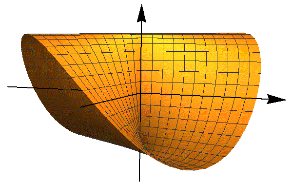
- f*(r,θ) = r sin(3θ), a linear function of t on each line (x,y) = (at,bt), but not differentiable at (x,y) = (0,0), the "crinkle" at (0,0) ruling out any good tangent plane.
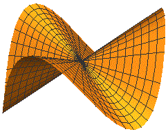
- f*(r,θ) = sin(2θ),
a function constant on each radial line (x,y) = (at,bt),
but not continuous at (x,y) = (0,0).
- Find the following limits lim(x,y)→(0,0) f(x,y), if they exist.
Hints:
- Freely use known facts about one-dimensional limits, such as L'Hopital's Rule.
- Ignore points where f(x,y) is undefined: we only care whether the defined values approach a limit.
- If we can write f(x,y) = g(h(x,y)), where g(t) is a one-variable function, the limit can be reduced to computing lim(x,y)→(a,b) h(x,y) = L, then limt→L g(t).
- To show a limit does not exist, find two curves (x(t), y(t)) such that f(x(t), y(t)) approaches different values as (x(t), y(t)) → (0,0).
- (p 103 #9) f(x,y) = (exy − 1)⁄y
- (p 103 #9) f(x,y) = (cos(xy) − 1)⁄x2y2
- (p 103 #6) f(x,y) = xy3⁄x2+y6 (Examine (x(t), y(t)) = (t,0) and (t3, t).)
- (p 103 #10) f(x,y) = (x−y)2⁄x2+y2
- (p 115 #7) Consider the tangent plane P of the graph z = f(x,y) = ex−y above the point (x,y) = (1,1).
- Find an equation for P of the form z = a + bx + cy. Hint: Write the graph of the affine approximation to f(x,y) near (x,y) = (1,1), and simplify.
- Find a vector q orthogonal to the plane P (that is, orthogonal to any vector between two points of P). Hint: Write the equation for P in the form (x,y,z) • q = d. Why is this q orthogonal to P?
- (p 115 #16) Use an affine approximation for the function f(x,y,z) = (x2 + y2 + z2)1/2 to find an accurate esimate of the number: = ((4.01)2 + (3.98)2 + (2.02)2)1/2
1a. f*(r,θ) = sin(2θ) = 2 sin(θ)cos(θ) = 2(r sin(θ))(r cos(θ))⁄r2 , corresponding to f(x,y) = 2xy⁄(x2+y2). Note that f(ta,tb) = 2ab⁄(a2+b2). Thus, although the function is identically zero along the x- and y-axes, it has a different constant value on each radial line of approach (ta,tb) as t→0; it has an essential discontinuity at (x,y) = (0,0).1b. f*(r,θ) = r sin(3θ) = r sin(θ)cos(2θ) + r cos(θ)sin(2θ) = 3r cos2(θ)sin(θ) − r sin3(θ) = 3(r cos(θ))2(r sin(θ))−(r sin(θ))3⁄r2 , corresponding to f(x,y) = y(3x2−y2)⁄(x2+y2). Note that f(ta,tb) = b(3a2−b2)⁄(a2+b2) t. Thus, although the function has gradient ∇f(0,0) = (∂f⁄∂x(0,0),∂f⁄∂y(0,0)) = (0,−1), the linear approximation L(h1,h2) ≈ f(0,0) + ∇f(0,0)•(h1,h2) = −h2 is not valid on each radial line of approach (h1, h2) = (ta,tb) as t→0. The function is non-differentiable at (x,y) = (0,0).
2a. f(x,y) = (exy − 1)⁄y = x (exy − 1)⁄xy = x (et − 1)⁄t , where t = xy. Since limt→0 (et − 1)⁄t = 1 by L'Hopital's Rule, we have lim(x,y)→(0,0) f(x,y) = (0)(1) = 0.
2b. Again taking t = xy and using L'Hopital twice gives lim(x,y)→(0,0) f(x,y) = (cos(t) − 1)⁄t2 = −½.
2c. Consider f(t,0) = 0, and f(t3, t) = t6⁄2t6 = ½. Thus no matter how close (x,y) is to (0,0), there are values of f(x,y) equal to 0, and others equal to ½, so f(x,y) does not approach a single limit value.
2d. We take f(t,t) = 0, and f(t, −t) = (2t)2⁄2t2 = 2, so again f(x,y) does not approach a single limit value as (x,y) → (0,0).
3a. For f(x,y) = ex−y, we have: ∂f⁄∂x|(x,y)=(1,1) = 1, and ∂f⁄∂y|(x,y)=(1,1) = −1, so the affine approximation is:
f(x,y) ≈ f(1,1) + ∂f⁄∂x (x−1) + ∂f⁄∂y (y−1) ≈ 1 + (x−1) − (y−1) ≈ 1 + x − y and the tangent plane is: z = 1 + x − y.
3b. The equation of P can be written as: −x + y + z = 1, i.e. (x,y,z) • (−1, 1, 1) = 1. Thus q = (−1, 1, 1) is orthogonal to the plane. Indeed, any two points v, v' on the plane satisfy v • q = v' • q = 1 so the vector v −v' between them, a vector parallel to the plane, has (v−v') • q = 1−1 = 0.
4. For (x,y,z) = (4.01, 3.98, 2.02) near (4,4,2), we have the affine linear approximation f(x,y,z) ≈ f(4,4,2) + ∇f(4,4,2) • (x−4, y−4, z−2) ≈ 6 + (2⁄3, 2⁄3, 1⁄3) • (x−4, y−4, z−2) = 6 + 2⁄3(x−4) + 2⁄3(y−4) + 1⁄3(z−4) = 6 + 2⁄3(0.01) + 2⁄3(−0.02) + 1⁄3(0.02).
- 11/15 Lect 33. ⊞ Taylor series f(a+h) = ∑Nn=0 f(n)(a)⁄n! hn + o(hN)
⊞ Solutions- Calc I review: Taylor Series
- Higher derivatives; equality of mixed partials:
∂2f⁄∂x∂y
=
∂2f⁄∂y∂x
provided both second deriv functions are continuous at (x,y) = (a,b) - Proof of Taylor's Theorem with remainder bound.
Repeated integration by parts of
f(a+h) = f(a) + ∫aa+h f '(t) dt = f(a) − ∫aa+h f '(t)(a+h−t)' dt
gives integral form:f(a+h) = f(a) + f '(a)h + f "(a)⁄2! h2 + · · · + f (k)(a)⁄k! hk + Rk(a,h), with remainder Rk(a,h) = 1⁄k! ∫aa+h f(k+1)(t) (a+h−t)k dt.
Thus, |Rk(a,h)| ≤ M |h|k+1⁄k!, where |f(k+1)(t)| ≤ M for t ∈ [a,a+h]. - Taylor Formula for f : R2 → R
f(a+h1,b+h2) = ∑i,j≥0 1⁄i!j! ∂fi+j⁄∂ix∂jy(a,b) h1i h2j
f(x,y) = ∑i,j≥0 1⁄i!j! ∂fi+j⁄∂ix∂jy(a,b) (x−a)i(y−b)j
Warning: Coefficients are constants involving (a,b), not functions of (x,y) - Quadratic term in Taylor approx given by Hessian matrix:
f(a+h) = f(a) + [Dfa]•h + 1⁄2 h•[Hfa]•hT + o(|h|2)
where h is 1×2 row-vector, [Hfa] is 2×2, hT is 2×1 column-vector
Equality of mixed partials ⇒ Hessian [Hf] is a symmetric matrix[Hfa] = ∂2f⁄∂x2(a) ∂2f⁄∂x∂y(a) ∂2f⁄∂y∂x(a) ∂2f⁄∂y2(a)
HW- Consider an iron bar marked with the
position coordinate x ≥ 0,
and let f(x,t) denote the temperature of position x at time t.
The Heat Equation is a partial differential equation
(i.e. a differential equation involving partial derivatives)
which models the flow of heat in the bar: the temperature f(x,t) must satisfy:
∂f⁄∂t = ∂2f⁄∂x2
Problem: Show that f(x,y) = 1⁄√t exp(− x2⁄4t) is a solution to the Heat Equation. Graph some slices z = f(x,t) above t = 0.1, 0.5, 1.0, 2.0 to see how the heat dissipates from a point-source at x = 0. - (Ch 3.1 p 157 #18) For f(x,y,z) = z exy + x2yz3, verify that:
∂3f⁄∂x∂y∂z = ∂3f⁄∂z∂y∂x
- Let f(x,y) = cos(xy).
- Give the quadratic Taylor approximation of f(x,y) centered
at (x,y) = (0,0),
f(h1,h2) ≈ c00 + c10 h1 + c01 h2 + 1⁄2(c20 h12 + c11 h1 h2 + c02 h22) for explicit constants c00, . . . ,c02.
Note: error term is o(|h2|) = o(h12+h22) as (h1,h2) → (0,0) - Use the infinite Taylor series for cos(t) at t = 0 to find the full Taylor series of f(x,y) at (x,y) = (0,0).
- Give the quadratic Taylor approximation of f(x,y) centered
at (x,y) = (0,0),
- (Ch 3.2 p 166 #11) Find the second-order Taylor polynomial (quadratic approximation) at (x,y) = (½π, 1) for the function:
f(x,y) = sin(xy) − 3x2 log(y) + 1. - (Ch 3.3 p 182 #5, 9, 19) Find the critical points of the following
functions, and use the Hessian to classify them as maximum, minimum, saddle,
or degenerate.
e1+x2−y2 , cos(x2+y2)
1⁄3 x3 + 1⁄3 y3 − 1⁄2 x2 − 5⁄2 y2 + 6y + 10.
Verify your conclusions by inspecting the contour plots or graphs of these functions. (This is the easiest way to classify the critical points, but it is only possible for two variables.) - The Positive-Definiteness Criterion (Lemma 2, p. 174−176) says that,
if we have a quadratic function defined by
a Hessian matrix:
q(x,y) = [x,y] • a b b c • [x,y]T = ax2 + 2bxy + cy2,
then q(x,y) is positive-definite, meaning q(0,0) = 0 and q(x,y) > 0 for (x,y) ≠ (0,0), whenever a > 0 and det(H) = ad − bc > 0.
Prove this by completing the square to get:q(x,y) = a(x + b⁄a y)2 + (ac−b2)⁄a y2.
For what a,b,c is this always positive?
1. See M&T p. 156, Example 6.3a. cos(h1h2) = 1 + o(h12+h22), since all the first and second partial derivatives become zero for (x,y) = (0,0). In fact, the first non-zero term is 1⁄2 h12h22.
3b. Using cos(t) = ∑n≥0 (−1)n⁄(2n)! t2n gives: cos(h1h2) = ∑n≥0 (−1)n⁄(2n)! h12nh22n
4. See p. 509.
5. See p. 510. Correction for #19: For f(x,y) = 1⁄3 x3 + 1⁄3 y3 − 1⁄2 x2 − 5⁄2 y2 + 6y + 10, the critical points are classified as:
(0,3) saddle, (1,2) saddle, (0,2) max, (1,3) min.
6. See p. 175.
- 11/18 Lect 34. ⊞ Properties of Derivative DF, Chain Rule
⊞ Solutions- Chain Rule: D(F◦G)a = DFG(a) ◦ DGa
Proof: Substitute linear approx of G into lin approx of F, show error is o(h)
HW- (p 133 #13) Suppose a duck is swimming in the circular path c(t) = (cos(t), sin(t)), and the water temperature is given by T(x,y) = x2ey − xy3. Find dT⁄dt in two ways: by the Chain Rule for T(c(t)), and by writing out the formula for f(t) = T(c(t)) and directly differentiating.
- Theorem: Consider the function f : R3 → R with the level surface S = {(x,y,z) with f(x,y,z) = d}. Suppose
c(t) = (x(t), y(t), z(t)) is a curve contained in the surface S,
with c(0) = (a,b,c). Then the tangent vector c'(0)
is orthogonal to the gradient ∇f(a,b,c).
Thus, the level surface S is orthogonal to the gradient.
Prove this Theorem by applying the Chain Rule to f(c(t)). - (p. 142 #4) You are walking on a hillside in the shape of the graph z = y cos(πx) − x cos(πy) + 10, standing at the point (2,1,13). Find an xy-vector direction you can walk so as to stay at the same level, a vector pointing along a contour. (How is this related to the uphill direction?)
- Consider the function f : R3 → R given by f(x,y,z) = x2 + 2y2 + 3z2.
- Describe the level surface S ⊂ R3 defined by f(x,y,z) = d, for a given constant d. (The level surface of a three-variable function is the analog of the level curve (contour) of a two-variable function.)
Hint: Consider the points with x2 + y2 + z2 = d, and modify the y- and z-coordinates to get f(x,y,z) = d. - Find the equation of the tangent plane to the surface f(x,y,z) = 13 at the point (1,0,2).
Hint: How does the level surface relate to the gradient vector ∇f(1,0,2), the direction of fastest increase of f? See M&T p. 139.
- Describe the level surface S ⊂ R3 defined by f(x,y,z) = d, for a given constant d. (The level surface of a three-variable function is the analog of the level curve (contour) of a two-variable function.)
1. For a function T(x,y) and a curve c(t) = (x(t), y(t)), the Chain Rule says:
dT⁄dt = d⁄dt T(c(t)) = ∇T(c(t)) • c'(t) = ∂T⁄∂x dx⁄dt + ∂T⁄∂y dy⁄dt . Plugging in the given functions to this formula gives the same result as first plugging in to get f(t) = T(c(t)), and then using the one-variable Chain Rule to compute f '(t).
2. Theorem: If a curve c(t) = (x(t),y(t),z(t)) goes along a level surface of the function f(x,y,z), then the tangent c'(t) is orthogonal to the gradient ∇f(c(t)).
Proof: By hypothesis, we assume f(c(t)) = a for all t and some constant a. Differentiating the left side by the multivariable Chain Rule gives:
d⁄dt f(c(t)) = d⁄dt( a ) ∇f(c(t)) • c'(t) = 0.
This confirms that the gradient is orthogonal to the tangent, as desired.
3. In the graph, z = f(x,y), the gradient ∇f(a,b) in the xy-plane points in the uphill direction from (a,b), which is always orthogonal to the contour curve (level curve) C = {(x,y) with f(x,y) = f(a,b)}. Thus, the orthogonal vector ∇f(a,b)⊥ points along the C at (a,b). Note: ∇f(a,b) has a unique orthogonal direction because it is a vector in the plane R2. (A three-dimensional vector has a whole plane of orthogonal vectors.)
4a. The points (x,y,z) with x2 + y2 + z2 = d form the sphere with radius √d from the origin. Squeezing these points to (x, y⁄√2, z⁄√3) gives the solutions to f(x,y,z) = d, namely the level surface S. Thus S is an ellipsoid: a sphere flattened by a factor of 1⁄√2 in the y direction, and by 1⁄√3 in the z direction.
4b. The gradient ∇f(a,b,c) ∈ R3 points in the direction of fastest increase of f(x,y,z), starting from (a,b,c). This is orthogonal to the directions of no increase, namely the tangents to the level surface. (Thinking of f(x,y,z) as temperature, the gradient points in the hottest direction, which is orthogonal to the directions of constant temperature.)
The plane orthogonal to q and passing through the point p is given by v = (x,y,z) satisfying q • (v−p) = 0, or equivalently q • v = q • p. Thus, the equation of the tangent plane to S is given by:
∇f(a,b,c) • (x,y,z) = ∇f(a,b,c) • (a,b,c) 2ax + 4by + 6cz = 2a2 + 4b2 + 6c2.
For (a,b,c) = (1,0,2), this is 2x + 12z = 26.
- 11/20 Lect 35. ⊞ Product Rules
⊞ Solutions- For F,G : Rk → Rn, dot product function F•G : Rk → R, (F•G)(v) = F(v)•G(v)
- Discover a Dot Product Rule by finding linear approximation at
v = a + h for
h → 0 ∈ Rk
(F•G)(a+h) = (F(a) + DFa(h) + o(h)) • (G(a) + DGa(h) + o(h))
= F(a)•G(a) + DFa(h)•G(a) + F(a)•DGa(h)
+ F(a)•o(h) + G(a)•o(h) + DFa(h)•o(h) + o(h)•DGa(a) + o(h)•o(h) - The error function on the last line is in the order-of-magnitude class:
o(h) = { ε : Rk → Rn with limh→0 |ε(h)|⁄|h| = 0 }, since all its terms and coordinates are in this class. For example, DFa(h) means an n×k Jacobian matrix times the k×1 column vector h = (h1, . . . , hk), making an n×1 column vector; so |DFa(h)| < C |h| where C is k times the largest (constant) matrix entry of DFa. Also |DFa(h)•o(h)| ≤ |DFa(h)| |h|. Therefore DFa(h)•o(h) ∈ o(1)o(h) = o(h). - Dot Product Rule:
Extracting the linear term from the above approximation, we find:
D(F•G)a(h) = DFa(h)•G(a) + F(a)•DGa(h). This is a linear function D(F•G)a(h) : Rk → R, so it has a 1×k derivative matrix, which we usually write as the gradient ∇(F•G)(a). - We can write this matrix using the matrix-transpose: if [v] denotes an
n×1 column vector, we write [v]T to mean the 1×n row vector; then we can express dot product in terms of matrix product as v•w = [v]T [w]. Then we have, in terms of matrix sums and products:
[D(F•G)a] = ∇(F•G)(a) = [G(a)]T [DFa] + [F(a)]T [DGa]. Here [G(a)]T is a 1×n row vector, matrix multiplied by the n×k Jacobian [DFa] to give a 1×k product matrix.
HW:- Apply the dot product derivative rule to the identity function I(v) = v, to find the gradient of ∇(v•v) = ∇|v|2.
- Apply the Chain Rule to find the gradient of |v|2c for any c ∈ R, in particular |v|.
- Derivative of f(v)G(v)
- Given f : Rk → R,
and G : Rk → Rn,
we can dilate the output G(v) by the scalar f(v),
forming the scalar-times-vector product function
f(v)G(v) or
f G : Rn → Rn.
Find a Scalar-times-vector Product Rule for this function by multiplying linear approximations at v = a+h, and computing the n×k Jacobian matrix D(fG)a. - Apply this Product Rule for G = I to find the derivative matrix of f(v) v for any f.
- Given f : Rk → R,
and G : Rk → Rn,
we can dilate the output G(v) by the scalar f(v),
forming the scalar-times-vector product function
f(v)G(v) or
f G : Rn → Rn.
- Extra Credit: Can you come up with a Cross Product Rule?
1. The identity function is a linear mapping, having the same n×n matrix as its Jacobian: DIa = I, the identity matrix with 1's on the main diagonal and 0's elsewhere, satisfying MI = M and/or IM = M whenever either multiplication is defined. Thus:∇(v•v)(a) = 2[I(a)]T DIa = 2[a]T I = 2[a]T. Writing v instead of a, this can be written as: ∇|v|2 = 2v. We can check this by differentiating directly:
∇|v|2 = ∇(x2+y2+z2) = (2x, 2y, 2z). 2. By the Chain Rule:
∇|v|2c = ∇(|v|2)c = c(|v|2)c−1 ∇|v|2 = c(|v|2)c−1 2v = 2c |v|2c−1 v⁄|v| . For c = 1⁄2, we get ∇|v| = v⁄|v| . Again, these formulas may be checked by direct differentiation.3a. To find the derivative of the scalar-times-vector product of functions, we plug in linear approximations for f(v) and G(v):
f(a+h) G(a+h) ≈ (f(a) + ∇f(a)•h) (G(a) + DGa(h)) The last term is proportional to |h|2, so it in o(h), and all other error terms are also in o(h) by the same reasoning as for the Dot Product Rule. The middle terms are linear in h, and give the derivative of the product.
= f(a) G(a) + f(a) DGa(h) + (∇f(a)•h) G(a) + (∇f(a)•h) DGa(h)Scalar-times-vector Product Rule:
D(fG)a(h) = f(a) DGa(h) + (∇f(a)•h) G(a) The n×k Jacobian matrix is thus:[D(fG)a] = f(a) DGa + G(a) ∇f(a). Here DGa is an n×k Jacobian matrix; and the last term is the product of the n×1 column vector G(a) and the 1×k row vector ∇f(a), making an n×k matrix.3b. For F(v) = f(v) v = f(v) I(v), we get the n×n Jacobian matrix:
[DFa] = f(a) DIa + I(a) ∇f(a) = f(a) I + a ∇f(a). Here I is the n×n identity matrix; and the last term is the n×1 column matrix a times the 1×n row matrix ∇f(a), giving an n×n matrix. Writing v instead of a:D(f(v)v) = f(v) I + v ∇f(v). - 11/21 Recitation 13. Line integral and curl in R3
- 11/22 Lect 36. ⊞ Gradient, line integral ∫ F(c)•dc, conservative F, curl in R3
⊞ Solutions- Gradient of f : R3 → R
Dfa = ∇f(a) = (∂f⁄∂x(a), ∂f⁄∂y(a), ∂f⁄∂z(a)) - Directional derivative: rate of change of f in direction
v with |v| = 1
∂f⁄∂v(a) = limh→0 (f(a+hv)−f(a))⁄h - Gradient geometric meaning:
∂f⁄∂v(a)
=
∇f(a) • v.
Also: ∇f(a) is the direction of maximum increase of f from a,
and |∇f(a)| is the maximum rate of increase of f at a.
Proof: Using the linear approximation to f near a:∂f⁄∂v(a) = limh→0 (f(a+hv)−f(a))⁄h = limh→0 1⁄h (f(a) + Dfa(hv) + o(h) − f(a)) Since |∇f(a) • v| = |∇f(a)| |v| cos(θ), the length |∂f⁄∂v(a)| is largest for θ = 0,= limh→0 1⁄h ∇f(a) • hv + o(h)⁄h = ∇f(a) • v.
i.e. v = ∇f(a)⁄|∇f(a)| , giving |∂f⁄∂v(a)| = |∇f(a) • v| = |∇f(a)|. - Vector field F : R3 → R3, F(x,y,z) = (p(x,y,z), q(x,y,z), r(x,y,z))
- Line integral ∫ F(c) • dc
= ∫10 F(c(t)) • c'(t) dt
Geometric meaning
How strongly F pulls along curve c
Negative if F pulls against direction of c
Physics meaning
Work done by force F in moving particle along c
= negative of work done by particle moving along c against force F - Gradient Theorem:
For F conservative, F = ∇f,
the line integral of F over c
equals the change in potential between endpoints a = c(0) and b = c(1):∫ ∇f(c) • dc = f(b) − f(a). Proof: Let g(t) = f(c(t)), so by the Chain Rule, g'(t) = Dfc(t) Dct = ∇f(c(t)) • c'(t).
Then the single-variable Second Fundamental Theorem of Calculus says:f(b) − f(a) = g(1) − g(0) = ∫10 g'(t) dt = ∫10 ∇f(c(t)) • c'(t) dt = ∫ ∇f(c) • dc. - Conservative Vector Field Theorem. The following are equivalent:
- Conservative: F = ∇f for some potential function f
- Path Independent: ∫ F(c1) • dc1 = ∫ F(c2) • dc2 for any curves dc1 and dc2 with same endpoints
- Zero Circulation: ∮ F(c1) • dc1 = 0 around any closed loop c with c(0) = c(1)
- Irrotational: curl F = 0 at every point (need to define curl F in higher dim)
(ii) ⇒ (i) follows from single-variable First Fundamental Theorem of Calculus over rectangular c.
(ii) ⇔ (iii) follows from cutting a loop into two opposite paths.
(iii) ⇒ (iv) follows from definition of curl F as rate of circulation
(iv) ⇒ (iii) follows from Curl Theorem (Stokes Theorem) - Higher dimensions: all the above is valid in Rn, for F(x1, . . . , xn) = (p1, . . . , pn)
- Curl in R3.
Vector field F(x,y,z) = (p(x,y,z), q(x,y,z), r(x,y,z))
Curl of F is vector of 2-dim curls of F around x,y,z axes (in coordinate planes yz, xz, xy):curl F = (curlyz(q,r), −curlxz(p,r), curlxy(p,q)) = (∂r⁄∂y − ∂q⁄∂z , ∂p⁄∂z − ∂r⁄∂x , ∂q⁄∂x − ∂p⁄∂y) Note that a rotation curling right-hand fingers from x to z has thumb axis in the negative y direction, which gives the negative sign on the curlxz coordinate. - Determinant formula for curl:
curl F = ∇×F = (∂⁄∂x ,∂⁄∂y ,∂⁄∂z) × (p, q, r) = det i j k ∂⁄∂x ∂⁄∂y ∂⁄∂z p q r - Directional curlv F(a)
for unit vector |v| = 1:
Rate of circulation of F at point a,
around axis v, in plane pependicular to v.
The directional curl equals the component of the vector curl in
direction v:
curlv F(a) = curl F(a) • v. Maximum rate of circulation is |curl F| in direction v = curl F⁄|curl F|
Direction of curl F(a,b,c) = axis of rotation of multi-directional paddlewheel
with center fixed at (a,b,c), under the flow F -
If F = ∇f is conservative, it has zero circulation,
so rate of circulation is zero in all directions:
curl F = curl ∇f = 0.
[MT] Ch 4.4 on Curl, odd ex p. 234; review Lect 14 on arclength.
Review Lect 15 on circulation in R2
HW:- Consider the vector field F(x,y,z) = (−x,−y,1).
- Make a rough sketch and verbal description of the arrows of F.
- Find a potential function f(x,y,z) with ∇f = F, by evaluating a line integral ∮ F(c)•dc over the straight line c from (0,0,0) to (a,b,c).
- Redo the above line integral over the curve c = (at, bt2, ct3) for t ∈ [0,1].
- Write an integral to compute the arclength of the curve c = (t, t2, t3) for t ∈ [0,1]. Get a numerical approximation from Wolfram Alpha.
- Consider the vector field F(x,y,z) = (−y,x,1).
- Make a rough sketch and verbal description of the arrows of F.
- Try to find a potential function f(x,y,z) with ∇f = F, by evaluating a line integral ∮ F(c)•dc over the straight line c(t) = (at,bt,ct) from (0,0,0) to (a,b,c). Check to see if the resulting function really has the desired gradient.
- Redo the above line integral over the curve c(t) = (at2, bt2, ct2) for t ∈ [0,1]. This is the same straight line, but traversed at a different speed. We say that this is a reparametrization of the original c(t) = (at,bt,ct).
- Try to express intuitively why the vector field is not conservative. (Compare to the two-variable case from Lect 14 & 15).
- For the two vector fields above, compute curl F and compare with your geometric intuition.
- Check by computation that curl ∇f(x,y,z) = (0,0,0) for any f.
Hint: Use equality of mixed partials: ∂⁄∂x∂⁄∂yf(x,y,z) = ∂⁄∂y∂⁄∂xf(x,y,z) , etc.
1a. The vector field F(x,y,z) = (−x,−y,1) points in toward the z-axis and tilts upward. Nearer the z-axis, the vectors get shorter and tilt up more, pointing straight up along the axis itself.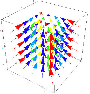
1b. Using the Gradient Theorem
f(a,b,c) − f(0,0,0) = ∮ F(c)•dc = ∫10 F(at,bt,ct) • (at,bt,ct)' dt = ∫10 (−at,−bt,1) • (a,b,c) dt Arbitrarily setting f(0,0,0) = 0, we get f(x,y,z) = −½x2 − ½y2 + z, which indeed gives ∇f(x,y,z) = (−x,−y,1) = F(x,y,z).= ∫10 −a2t − b2t + c dt = −½a2t2 − ½b2t2 + ct |1t=0 = −½a2 − ½b2 + c.
1c. We have:
f(a,b,c) = ∫10 F(at, bt2, ct3) • (at, bt2, ct3)' dt = ∫10 (−at, −bt2, 1)•(a, 2bt, 3ct2) dt giving the same f(x,y,z) = −½x2 − ½y2 + z as before. This is expected because of the Gradient Theorem, which guarantees that a gradient vector field is path-independent, depending only on the enpoints of the path of integration.= ∫10 −a2t − 2b2t3 + 3ct2 dt = −1⁄2a2t2 − 2⁄4b2t4 + ct3 |1t=0 = −½a2 − ½b2 + c,
1d. L = ∮ |dc| = ∫10 |c'(t)| dt = ∫10 |(1, 2t, 3t2)| dt = ∫10 √(1 + 4t2 + 9t4) dt ≈ 1.86 , slightly longer than the straight-line path with length |(1,1,1)| = √3 ≈ 1.73 .
2a. The vector field F(x,y,z) = (−y,x,1) rotates around the z-axis (with right-handed orientation) and tilts upward. Nearer the z-axis, the vectors get shorter and tilt up more, pointing straight up along the axis itself.
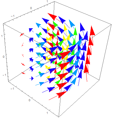
2b. F(c)•dc = ∫10 F(at,bt,ct) • (at,bt,ct)' dt = ∫10 (−bt,at,1) • (a,b,c) dt = ∫10 −bat + abt + c dt = ct |1t=0 = c. Thus f(x,y,z) = z gives ∇f(x,y,z) = (0,0,1), which is not F(x,y,z) = (−y,x,1). Thus, F cannot be a conservative vector field: there is no potential function.
2c. ∫10 F(at2, bt2, ct2) • (at2, bt2, ct2)' dt = ∫10 (−bt2, at2, 1)•(2at,2bt,2ct) dt = ∫10 2ct dt = ct2|1t=0 = c. This gives the same function f(x,y,z) = z as in part (b).
In fact, even if the vector field is non-conservative, and the line integral changes upon changing the path between fixed endpoints, nevertheless the line integral is unchanged upon reparametrizing the same curve. We say that line integrals are always parametrization independent, even if they are not path independent.
2d. The vector field is not conservative because its vortex pattern has non-zero circulation, and thus gives different line integrals along the two halves of a loop. In the next lecture, we will define curl F, and see it is non-zero.
3. For the first vector field, we use the determinant formula to compute curl(−x,−y,1) = (0,0,0). This makes sense from the picture, since for any small rectangle in a coordinate plane, F is either perpendicular to it, or pushes along opposite sides equally, making zero circulation near every point.
For the second vector field, we have curl(−y,x,1) = (0,0,2), which matches the rotation of F around the z-axis in the picture. Also, you can use the right-hand rule to determine the polarity of the rotation axis: if you curl your fingers in the direction of rotation, your thumb points upward in the positive z-direction, agreeing with curl F = +2k.
4. This is a straightforward computation, plugging F = (p,q,r) = (∂f⁄∂x , ∂f⁄∂y , ∂f⁄∂z) into the formula for curl F.
- 11/25 Lect 37. ⊞ Directional curl
⊞ Solutions- Directional curl. Recall curl of 3D vector field F = (p,q,r):
curl F = ∇×F = (∂r⁄∂y − ∂q⁄∂z , ∂p⁄∂z − ∂r⁄∂x , ∂q⁄∂x − ∂p⁄∂y). For a plane near a point a spanned by basis vectors u,v, define directional curl to mean the rate of circulation of F around a small curve c(t) in the given plane, per unit area enclosed:curluv F = limc→a 1⁄area(c) ∮ F(c) • dc . - Theorem:
The directional curl is equal to the component of the vector curl perpendicular to the plane:
curluv F = (curl F) • n⁄|n| , where n = u×v is the normal vector of the plane, and n⁄|n| is the unit normal vector.
Proof: For h > 0, consider the parallelogram curve ch(t) defined by the four linear segments:a + tu , a + u + tv , a + (h−t)u + v , a + (h−t)v , each running over t ∈ [0,h]. The area enclosed is the length of the cross product |hu × hv| = h2|u×v|, and we compute:curluv F = limh→0 1⁄h2|u×v| (∫01 F(a+tu) • u dt + ∫01 F(a+u+tv) • v dt + ∫01 F(a+(h−t)u+v) • (−u) dt + ∫01 F(a+(h−t)v) • (−v) dt). Substituting F(a + r(t)) = F(a) + DFa(r(t)) + o(h), and writing DF(u) • v in terms of matrix products as uT DFT v, where u, v are considered as column vectors, we compute the limit:1⁄|u×v| (uT DFT v − v DFT u) = 1⁄|u×v| uT(DFT−DF)v The above applies to a parallelogram curve, but the Theorem holds for arbitrary c(t) converging to a in the plane of u,v.
= 1⁄|u×v| det(curl F, u, v) = (curl F) • u×v⁄|u×v| .
- Consider the vector field F(x,y,z) = (0,0,x+y).
- Compute the vector curl F
- Compute the directional curl around the coordinate axes i, j, k (i.e. along the planes perpendicular to these vectors).
- Around what direction is the directional curl maximal?
- Sketch F and verify the above computations geometrically.
Hint: Draw the arrows F(x,y,0) from the xy coordinate plane.
1a. The determinant formula gives: curl F = (1,−1,0).1b. The directional curls around the x,y,z axes are the components of the vector curl: curl(1,0,0) = 1, curl(0,1,0) = −1, curl(0,0,1) = 0.
1c. For a direction v with |v| = 1, the directional curl around the axis v is:
curlv F = (curl F) • v = |curl F| |v| cos(θ) This is maximal when the angle θ = 0, so that v = curl F⁄|curl F|, i.e. in the direction of the vector curl.1d.
The vector field, being independent of z, has the same vectors on each horizontal plane.
At every point, the main rotation is around the direction (1,−1,0). This is evident on the line y = x itself, but is also true on lines like y = x + 1, since the arrows get longer at points farther from y = x.
- 11/27 Lect 38. ⊞ Extra: Complex functions, conformal mappings, plane vector fields
- Complex numbers: algebra
- C = {a+bi for a,b ∈ R} with i2 = −1 and all usual properties of arithmetic (distributive, commutative, etc.)
- Multiplication rule is forced by distributivity: (a+bi)(c+di) = (ac−bd) + (ad+bc)i
- Define 1⁄(a+bi) = c+di where
(a+bi)(c+di) = 1 = 1+0i
Rationalize denominator with conjugate radical: 1⁄(a+bi) = (a−bi)⁄(a2+b2) = a⁄(a2+b2) − b⁄(a2+b2) i. - Fundamental Theorem of Algebra: Any polynomial f(x), with real or complex coefficients, has a root z ∈ C, a solution of f(z) = 0.
- Thus, adjoining further square roots or other algebraic quantities does not enlarge C; for example √(−3) = (√3)i . That is, C is the largest possible number system having all the properties of the real and rational numbers.
- Complex numbers: geometry
- The complex plane pictures vectors (a,b) ∈ R2 as numbers a+bi ∈ C. Every real number line or axis has its complex extension lurking around it.
- Complex multiplication of z,w ∈ C multiplies their lengths, and adds their angles.
- Complex multiplication linear mapping: for c = a+bi, z = x+iy,
define Mc : R2 → R2
by Mc(z) = cz. Matrix:
[Mc] = [
]a −b b a - For c with radius r and angle θ
from pos real axis, get
[Mc] = (r I) Rotθ dilation times rotation
Mapping Mc preserves angles, though not lengths
- Complex analytic function f(z) is a polynomial or a Taylor series (infinite polynomial)
- Defined in terms of complex addition & multiplication, so defined for all z ∈ C
- Derivative Dfc = Mf '(c), where f '(z) is the complex derivative (zn)' = nzn−1, exp'(z) = exp(z), etc.
- Conformal property: Dfc preserves angles between tangent vectors, so f(z) preserves angles between intersecting curves in complex plane
- Under f : C → C, standard grid in (v+ui)-plane goes to curvy grid in (x+yi)-plane with all crossings 90°!
- Examples:
Input coordinates: for the first mapping, we take z in the upper half-plane; for the second, |z| ≥ 1.f(z) = z2 f(z) = 1⁄z f(v+ui) = (v2−u2) + (2vu)i f(v−ui) = v⁄(v2+u2) + u⁄(v2+u2) i 
All curves intersect at right angles. - Consider the mapping f(z) = z2,
f(v+iu) = (v2−u2) + (2vu)i,
with inverse function:
g(w) = √w = √(r cos(θ) + i r sin(θ)) = √r cos(θ⁄2) + √r sin(θ⁄2), g(x+iy) = v + iu = 1⁄2sgn(y)√(x+√(x2+y2)) + 1⁄2√(−x+√(x2+y2)). In electrostatics, if we take the ray with u = 0 to be a side view of a half-plane of uniform negative charge, then u(x,y) is the electric potential energy, and E = −∇u(x,y) = −∇v(x,y)⊥ is the corresponding electric field.
- 11/28 & 29 Thanksgiving break, no recitation or lecture
- 12/2 Lect 39. ⊞ Curl Theorem (Stokes' Thm) ∫S(curl F)•dS = ∮ F(c)•dc
⊞ Solutions- Motivation for Curl Theorem. As in two dimensions, the total circulation of a vector field F around a curve c should be equal to the integral of the rate of circulation over any surface S enclosed by c.
- What do we mean by the "integral of the rate of circulation"?
- Surface S = P(S*) ⊂ R3 parametrized by P(u,v) = (x(u,v), y(u,v), z(u,v)) over parameter region S* ⊂ R2, with c(t) going around the boundary or edge of S.
- Tangent plane of S has basis
∂P⁄∂u ,
∂P⁄∂v .
Normal vector n(u,v) = ∂P⁄∂u × ∂P⁄∂v perpendicular to S at each point P(u,v) - Integral of rate of circulation is:
∬S* ( where we use the "vector surface area element" dS = n du dv.
) (curl F in tangent plane of S
) du dv = ∬S* (curl F) • n⁄|n| |n| du dvarea stretch factor of P
= ∬S* (curl F) • n du dv = ∬S (curl F) • dS, -
Curl Theorem (Stokes' Theorem): The integral of the rate of circulation of F over a surface S is equal to the total circulation around the boundary curve of S. That is, if a surface S = P(S*) has boundary curve c, then
∬S F • dS = ∮ F(c) • dc,
∬S* F(P(u,v)) • (∂P⁄∂u×∂P⁄∂v) du dv = ∫01 F(c(t)) • c'(t) dt.
- Justification: Line integral around the boundary of S is equal to the sum of line integrals around small parameter boxes making up S: line integrals along opposite internal boundaries cancel, leaving only external boundary contributions. The circulation around each parameter box is approximately directional curl times area (by definition), and this is given by (curl F)•n, as described above.
HW: Look at WHW 11 due 12/11 below.- Let S = hemisphere x2+y2+z2 = 1, x ≥ 0, from Lect 40 example,
and take F(x,y,z) = (0, 0, y(z+1)).
- Parametrize S by P(u,v) with P : S* → S, and find its normal vector n(u,v).
- Compute curl F.
- Compute the flux integral of curl F through S: that is ∬S curl F • dn = ∬S* F(P(u,v)) • (∂P⁄∂u×∂P⁄∂v) du dv.
- Parametrize the circular boundary of S by c(t), and compute its tangent vector c'(t).
- Compute the circulation of F around c, that is ∮ F(c) • dc, and verify that it gives the same answer as the double integral (c).
- Consider the tilted ellipse surface S
along the plane z = x+1 and inside the cylinder
x2 + y2 ≤ 1.
Also let F(x,y,z) = (−y,x,z).
- Parametrize S and its boundary curve c. Hint: First write the x- and y-coordinates of P(u,v) = (x(u,v), y(u,v), z(u,v)), then find z.
- Find the normal vector n(u,v) for S, and the tangent vector c'(t).
- Compute the total circulation of F around c.
- Compute the flux of curl F across S. By the Curl Theorem, this should the same as the circulation of F around the boundary curve in part (c).
1a. The spherical coordinate parametrization of the vertical half-sphere is:P(φ,θ) = (sin(φ) cos(θ), sin(φ) sin(θ), cos(φ)) for 0 ≤ φ ≤ π , −π⁄2 ≤ θ ≤ π⁄2 . Normal vector: n = ∂P⁄∂φ×∂P⁄∂θ = (sin2(φ)cos(θ), sin2(φ)sin(θ), sin(φ)cos(φ))1b. For F(x,y,z) = (0, 0, y(z+1)), we have:
curl F(x,y,z) = (∂⁄∂y(y(z+1)) − ∂⁄∂z(0), −∂⁄∂x(y(z+1)) + ∂⁄∂z(0), ∂⁄∂x(0) − ∂⁄∂y(0)) = (z+1, 0, 0). 1c. The integral of the curl over the surface is: ∬S curl F • dn
= ∫ −π/2 π/2 ∫ 0 π curl F(sin(φ)cos(θ), sin(φ)sin(θ), cos(φ)) • n(φ,θ) dφ dθ
= ∫ −π/2 π/2 ∫ 0 π (cos(φ)+1, 0, 0) • (sin2(φ)cos(θ), sin2(φ)sin(θ), sin(φ)cos(φ)) dφ dθ
= ∫ −π/2 π/2 ∫ 0 π (cos(φ)+1) sin2(φ) cos(θ) dφ dθ
= (∫ −π/2 π/2 cos(θ) dθ) (∫ 0 π (cos(φ)+1) sin2(φ) dφ) = (2)(π⁄2) = π.1d. The vertical boundary circle ∂S, with equations x = 0 and y2+z2 = 1, is given parametrically by c(t) = (0, cos(t), sin(t)) for 0 ≤ t ≤ 2π. Note that in curling the fingers of my right hand around c, my thumb points along the positive x-axis, which is the positive direction for S. The tangent vector is c'(t) = (0, −sin(t), cos(t)).
1e. The circulation around the boundary is: ∮ F(c) • dc
= ∫02π F(0, cos(t), sin(t)) • (0, cos(t), sin(t))' dt
= ∫02π (0, 0, cos(t)(sin(t)+1)) • (0, −sin(t), cos(t)) dt
= ∫02π cos2(t)(sin(t)+1) dt = π.
This agrees with part (c), as it must by the Curl Theorem.2a. Cylindrical coorinates: P(r,θ) = (r cos(θ), r sin(θ), r cos(θ) + 1) for 0 ≤ r ≤ 1 and 0 ≤ θ ≤ 2π. The boundary is: c(t) = (cos(t), sin(t), cos(t)+1) for 0 ≤ t ≤ 2π.
2b. n(r,θ) = ∂P⁄∂r × ∂P⁄∂r = (cos(θ), sin(θ), cos(θ)) × (−r sin(θ), r cos(θ), −r sin(θ)) = (−r, 0, r). The normal vector function is so simple because S lies in a plane orthogonal to (−1, 0, 1). The length |n| is the stretching factor of the parametrization: the grid boxes of P have size proportional to the radius r.
The tangent vector of the curve is: c'(t) = (−sin(t), cos(t), −sin(t)).
2c. ∮ F(c) • dc = ∫02π F(cos(t), sin(t), cos(t)+1) • (cos(t), sin(t), cos(t)+1)' dt = ∫02π (−sin(t), cos(t), cos(t)+1) • (−sin(t), cos(t), −sin(t)) dt • (cos(t), sin(t), cos(t)+1)' dt = 2π.
2d. We have curl F = (0,0,2), meaning that near every point, F primarily rotates around a vertical axis. The flux of the curl through S is:
∬S F × dn = ∫01 ∫02π (0,0,2) × (−r, 0, r) dθ dr = ∫01 4πr dr = 2π, which agrees with part (c), confirming the Curl Theorem in this case.- 12/4 Lect 41. ⊞ Flux, Divergence Theorem ∫∫∫R(div F) dV = ∬S F•dS
⊞ Solutions- Parametric surface S = P(S*) for P(u,v) = (x(u,v),y(u,v),z(u,v))
Normal vector n = ∂P⁄∂u × ∂P⁄∂v - Orientation of S designates positive normal direction n
- Flux of vector field F across oriented surface S:
Net flow of F from negative to positive side of S∬S F • dS = ∬S* F(P(u,v)) • n(u,v) du dv Justification: Flux = ∬S F • n⁄|n| |n| du dv, where:
F • n⁄|n| = component of flow perpendicular to S (i.e. across surface S)
|n| = |∂P⁄∂u×∂P⁄∂v| = area stretching factor of parameterization P(u,v) - Ex: S = unit hemisphere x2+y2+z2 = 1 , x ≥ 0
Parametrize: P(φ,θ) = (sin(φ)cos(θ), sin(φ)sin(θ), cos(φ)) for 0 ≤ φ ≤ π , −π⁄2 ≤ θ ≤ π⁄2
Normal vector: n = ∂P⁄∂φ×∂P⁄∂θ = (sin2(φ)cos(θ), sin2(φ)sin(θ), sin(φ)cos(φ)), points outward
Vector field F(x,y,z) = (0,0,z+1), pointing upward on S, getting longer as you go up
Net flow is positive: weak inflow of F through bottom of S, stronger outflow through top
Compute: net flow of F through S = ∬S F • dn = ∬S* F(P(u,v)) • n(u,v) du dv
= ∬S* F(sin(φ)cos(θ), sin(φ)sin(θ), cos(φ)) • (sin2(φ)cos(θ), sin2(φ)sin(θ), sin(φ)cos(φ)) du dv
= ∬S* (0, 0, cos(φ)−1) • (sin2(φ)cos(θ), sin2(φ)sin(θ), sin(φ)cos(φ)) du dv
= ∫ −π/2 π/2 ∫ 0 π (cos(φ)−1) sin(φ) cos(φ) dφ dθ = 2⁄3- Divergence of F means rate of flux of F across a small closed sufrace S near a, per unit area enclosed.
div F = limS→a ∬S F•dS / vol(S). In coordinates: F(x,y,z) = (p(x,y,z), q(x,y,z), r(x,y,z))div F = ∂p⁄∂x + ∂q⁄∂y + ∂r⁄∂z = (∂⁄∂x , ∂⁄∂y , ∂⁄∂z) • (p,q,r) = ∇ • F. - Divergence Theorem (Gauss' Theorem): The integral of the rate of flux of F over a solid region R is equal to the total flux of F outward across its boundary S. That is, if a solid region R = G(R*) has boundary surface S = P(S*), then
∫∫∫R (div F) dV = ∬S F • dS, or more explicitly:∫∫∫R* (div F)(G(u,v,w)) det[DG] du dv dw = ∬S* F • (∂P⁄∂u×∂P⁄∂v) du dv. - Justification: Flux integral across the boundary surface S is equal to the sum of flux integrals out of small parameter boxes making up R: flux integrals across common internal boundaries cancel, leaving only external boundary contributions. The flux out of each parameter box is approximately div F times volume (by definition), and this is given by div F.
- Divergence of F means rate of flux of F across a small closed sufrace S near a, per unit area enclosed.
Ch 7.6 Surface Integrals of Vector Fields, p. 400.
Ch 8.4 Gauss' Theorem, p. 461.
HW:- Divergence Theorem.
Consider the solid region R under the above plane
z = x+1, above the yz-plane, and inside the cylinder
x2 + y2 ≤ 1,
the shape of a wedge cut out of a tree-trunk:
R = {(x,y,z) | x2 + y2 ≤ 1 , 0 ≤ z ≤ x+1}. Again let F(x,y,z) = (−y,x,z).- Parametrize R and its three boundary surfaces, the top S1, side S2, and bottom S3. (The top is the same ellipse as in #1.)
- Compute the stretching factor det[DQ(u,v,w)] of the parametrization Q(u,v,w) of region R.
- Compute the normal vectors n(u,v) for S1, S2, S3. You might have to take negative of a normal to make sure it points out from R.
- Compute the total flux of F across the three surfaces.
- Compute the integral of div F on R. By the Divergence Theorem, this should the same as the flux of F across the boundary surfaces in part (d).
1a. R is parametrized in cylindrical coordinates by Q(r,θ,z) = (r cos(θ), r sin(θ), z) over the parameter region:R* = {(x,y,z) | 0 ≤ r ≤ 1 , 0 ≤ θ ≤ 2π , 0 ≤ z ≤ r cos(θ) + 1}. Here the z-range is defined by floor and ceiling functions depending on the previous variables r, θ.The top surface S1 is the same as S from the previous HW, P1(r,θ) = (r cos(θ), r sin(θ), r cos(θ) + 1) for 0 ≤ r ≤ 1 and 0 ≤ θ ≤ 2π.. The side surface S2 is defined by P2(θ,z) = (cos(θ), sin(θ), z) over S2* defined by 0 ≤ θ ≤ 2π and 0 ≤ z ≤ cos(θ)+1. The bottom surface S3 is the unit disk P3(r,θ) = (r cos(θ), r sin(θ) over S3* defined by 0 ≤ r ≤ 1 and 0 ≤ θ ≤ 2π.
1b. The stretching factor of Q(r,θ,z) is the determinant of its Jacobian matrix, i.e. the volume of the parallelopiped spanned by the gridline tangent vectors ∂Q⁄∂r, ∂Q⁄∂θ, ∂Q⁄∂z. This works out to det[DQ] = r, the same as for polar coordinates, since the z direction is not stretched at all.
1c. The normal vector of S1 is dn1 = (−r, 0, r), which correctly points upward (outward from R). The normal vector of S2 is dn2 = (cos(θ), sin(θ), 0), which points outward. The normal vector of S3 seems to be (cos(θ), sin(θ), 0) × (−r sin(θ), r cos(θ), 0) = (0, 0, r), but this points upward into R, so we must use its outward-pointing negative: n3 = (0, 0, −r).
1d. The total flux of F over the top surface is: ∬S2 F • dn2 = ∬S1* F(P1(r, θ)) • n1(r,θ) dr dθ = ∫01 ∫02π (−r sin(θ), r cos(θ);, r cos(θ) + 1) • (−r, 0, r) dr dθ = π.
From drawing R and F, we can see that F is parallel to the surface along S2 and S3, so it has no flux through these surfaces. This can be confirmed by calculating ∬S2 F • dn2 = ∬S3 F • dn3 = 0. Therefore the total flux over the surface ∂R = S1 ∪ S2 ∪ S3 is π + 0 + 0 = π.
1e. We have div F = ∂⁄∂x(−y) + ∂⁄∂y(x) + ∂⁄∂z(z) = 1. That is, F has a constant rate of flux from every point, due to the smaller inflow at the bottom of a small box than the outflow at the top.
Thus ∭R div F dx dy dz = ∭R* 1 det[DQ] dz dθ dr = ∫01 ∫02π ∫0r cos(θ)+1 r dz dθ dr = π, which agrees with (d), confirming the Divergence Theorem in this case.- 12/5 Recitation 15. Divergence Theorem
- 12/6 Lect 42. Extra review material. ⊞ Syllabus
- Geometric objects
- Vectors v = (x1, . . . , xn) ∈ Rn,
with addition, subtraction, scalar multiplication
Dot product: u•v = |u| |v| cos θuv
Cross product for v = (x,y,z): (u×v) • w = det(u,v,w), |u×v| = |u| |v| sin θuv - Curve C ⊂ Rn parametrized by c : R → Rn, c(t) over t ∈ [a,b], c(t) = (x1(t), . . . , xn(t))
- Region R ⊂ Rn
(plane or solid) with boundary ∂R,
points (x1, . . . , xn) ∈ R defined by:
- Simple region (successive floor/ceiling):
Plane: a ≤ x ≤ b , c(x) ≤ y ≤ d(x)
Space: a1 ≤ x ≤ b1 , a2(x) ≤ y ≤ b2(x) , a3(x,y) ≤ z ≤ b3(x,y)
General: a1 ≤ x1 ≤ b1 , a2(x1) ≤ x2 ≤ b2(x1) , a3(x1,x2) ≤ x3 ≤ b3(x1,x2) , . . . - Coordinate parameter function P : Rn → Rn
over simple parameter region u ∈ R*
P(u1, . . . ,un) = (x1(u1, . . . ,un), . . . , xn(u1, . . . ,un)) - Inequality defining region: f(x1, . . . , xn) ≤ c, with boundary contour f(x1, . . . , xn) = c
- Simple region (successive floor/ceiling):
- Surface S ⊂ R3
with boundary curve ∂S, defined by:
- Parameter function
P : R2 → R3,
P(u,v) = (x(u,v), y(u,v), z(u,v))
over simple parameter region (u,v) ∈ S* - Contour equation f(x,y,z) = c, cut off by inequalities g(x,y,z) ≤ a.
- Parameter function
P : R2 → R3,
P(u,v) = (x(u,v), y(u,v), z(u,v))
- Parametrized k-dimensional "surface" S ⊂ Rn
- P : Rk → Rn, P(u1, . . . , uk) = (x1, . . . , xn)
- S = P(S*) for parameter region S* ⊂ Rk
- Vectors v = (x1, . . . , xn) ∈ Rn,
with addition, subtraction, scalar multiplication
- Functions
- Scalar function f : Rn → R, gives number at each point (e.g. height, temperature, potential energy)
- General parameter function P : Rk → Rn
- Vector field F : Rn → Rn, arrow at each point (flow velocity, force)
- Derivative operations
- Nabla ∇ = (∂⁄∂x1 , ∂⁄∂x2 , . . . )
- Partial derivative ∂f⁄∂xi , grad f(x1, . . . ,xn) = ∇f
= ∂f⁄∂x1 +
· · · + ∂f⁄∂xn
Linear approximation: f(a+h) = f(a) + ∇f(a)•h + o(h)
Directional derivative ∂f⁄∂v = ∇f • v for |v| = 1 - Total derivative of P(u1, . . . , uk)
= (x1, . . . , xn)
- Linear function DPa : Rk → Rn, P(a+h) = P(a) + DPa(h) + o(h)
- Jacobian matrix (m rows) × (n columns):
[DPa] = [∂P⁄∂u1 | . . . | ∂P⁄∂uk ] =− ∇x1 − ⋮ − ∇xn −
- Hessian second-derivative matrix
- Hessian n×n matrix H(a) = [ ∂2f⁄∂xi∂xj(a) ]
- Quadratic Taylor series approximation
f(a+h) = f(a) + ∇f(a)•h + 1⁄2hT•H(a)•h + o(|h|2)
for n×1 column vector h and 1×n row vector hT
- Divergence div F = ∇ • F = ∂f1⁄∂x1 + · · · + ∂fn⁄∂xn for F = (f1, . . . , fn)
- Planar curl of F = (p,q): curl F = curl(p,q) = ∂q⁄∂x
−
∂p⁄∂y
Spatial curl of F = (p,q,r): curl F = ∇ × F = (curlyz(q,r), −curlxz(p,r), curlxy(p,q)) - Tangent vectors from parameter functions: c'(t) or ∂P⁄∂u1 , . . . , ∂P⁄∂uk
- Derivative of combination: Product Rules, Chain Rule
Obtained from product or composition of linear approx
- Integral operations
- Arclength ∫C dC = ∫ab |c'(t)| dt
- Line integral ∫C F • dC
= ∫ F(c(t)) • c'(t) dt, work done by F pulling along c;
For closed loop C, this is called circulation: ∮C F • dC - Size of a region
- Planar area ∫∫R dA = ∫∫R* |det[DP]| du dv
- Spatial volume ∫∫∫R dV = ∫∫∫R* |det[DP]| du dv dw.
- Surface area ∫∫S dA = ∫∫S* |dS| = ∫∫S* |∂P⁄∂u×∂P⁄∂v| du dv
- Flux integral: net flow of F across boundary,
toward right-hand or outward normal n
- Planar ∫C F • dn = ∫ab F(c(t)) • (−c'(t)⊥) dt
- Spatial ∫∫S F • dS = ∫∫S* F(P(u,v)) • (∂P⁄∂u×∂P⁄∂v) du dv
- Fundamental Theorems of Calculus
- Gradient Theorem: The integral of the rate of change of f along C is equal to the total change of f between the endpoints: ∫C ∇f • dC = f(b) − f(a), for C from a to b.
- Curl Theorem (Stokes):
The integral of the rate of circulation of F
over a surface
is equal to the total circulation of F around the boundary curve C.
- Planar ∫∫R curl F dA = ∮C F • dC
- Spatial ∫∫S curl F • dn = ∮C F • dC
- Divergence Theorem (Gauss): The integral of the rate of flux of F over a region is equal to the total flux of F out across the boundary.
- Planar ∫∫R div F dA = ∮C F • dn, C is boundary curve of R
- Spatial ∫∫∫R div F dV = ∫∫S F • dS, S is boundary surface of R
- Conservative Vector Field Theorem: The following conditions are equivalent for a vector field F:
- Conservative: There is a potential function f with ∇f = F.
In this case, f(a) = f(0) + ∫C F • dC for any curve C from 0 to a. - Path independent: ∫C1 F • dC1 = ∫C2 F • dC2 for any curves C1, C2 between the same endpoints.
- Zero circulation: Around any closed loop C, ∮C F • dc = 0.
- Irrotational: curl F(v) = 0 at all v
- Conservative: There is a potential function f with ∇f = F.
- Max/min of f : Rn → R over region R
- Critical point inside R: solve ∇f(v) = 0, for v ∈ R
- Parametrize boundary S = P(S*), critical points ∇f(P(u)) = 0
- Also consider endpoints of parametrized curve
- Choose absolute max & min values among f(v) for all critical & end points v
⊞ Problems I: Vector algebra, vector fields, potential, Jacobian derivative⊞ Solutions- Vector algebra. Consider the plane containing
(endpoints of) the vectors
a = (0,1,1), b = (1,1,0), c = (2,2,2).
- Find a parametric equation P(u,v) = (x(u,v), y(u,v), z(u,v)) for the plane.
- Find an equation for the plane as a level surface: ax + by + cz = d. (You will need a normal direction vector n, orthogonal to the directions along the plane.)
- Find the area of the triangle △abc, which is half the area of an appropriate parallelogram.
- Find the distance from the origin to the above plane. (Take a vector from the origin to the plane, and project it to the normal direction n.)
- Find the volume of the tetrahedron with vertices 0,a,b,c as 1⁄3 the area of the base triangle in part (c), times the height from part (d).
- Find the above tetrahedron volume another way, as 1⁄6 the volume of the parallelopiped spanned by edges a,b,c.
- Line integrals. Consider the vector field F(x,y) = (2x, 1).
- Sketch the field F, plotting sample vectors at grid points.
- Does it look like F is the gradient field (uphill vectors) of a potential function, i.e. F = ∇f? Sketch the contour lines and graph of this hypothetical f(x,y).
- Review the arguments from WHW 5 that F is conservative (having a potential function) if and only if it is irrotational (zero curl).
- Gradient Theorem: F = ∇f ⇒ f(c(1)) = f(c(0)) + ∮F(c)•dc is path independent (depends only on endpoints).
- ∮F path independent ⇔ F has zero circulation (∮F = 0 on any closed loop)
- Curl Theorem: F has zero circulatiion ⇐ curl F = 0 everywhere.
- Recall the pictorial meaning of curl F, why curl(0,x) = 1, curl(y,0) = −1, and curl(p,q) = ∂q⁄∂x − ∂p⁄∂y .
- Compute curl F.
- Compute f(a,b) = ∮ F(c)•dc = ∫10 F(c(t))•c'(t) dt for the straight line c(t) = (ta,tb) from (0,0) to (a,b). Compare to (b) above.
- Linear mappings and matrices
- Let R0 : R2 → R2 be the 1⁄4 counterclockwise rotation. Write its 2×2 matrix [ R0 ] = [ R0(i) | R0(j) ].
- In R3, compute the 3×3 matrix of a 1⁄4 rotation Rz around the z-axis, and similarly Rx around the x-axis.
- Multiply matrices to calculate the composite mapping: [Rz∘ Rx] = [ Rz ] • [ Rx ].
- Picture Rz∘ Rx by its effect on the unit vectors i, j, k, and describe it as a rotation.
- Consider the mapping f :
R2 → R3
defined by f(v) = (|v|, |v−i|,
|v−j|), recording the distances from v
to the origin and the two coordinate vectors.
- Find the Jacobian matrix of f at c = (½, 0), and write the affine linear approximation for f(x,y) near this point.
- Explain the form of the Jacobian geometrically: how could you have approximately predicted [ Df(c) ] without computing?
- For g(x,y,z) = x+y+z, use the Chain Rule compute the Jacobian matrix of
g∘f, and check that ∇(g∘f)(v) =
v⁄|v| +
v−i⁄|v−i| +
v−j⁄|v−j|.
Extra Credit: Show the sum of distances g(f(v)) is minimized when the three vectors v, v−i, v−j are all 120° from each other.
1a. Subtracting any two points on the plane P gives a direction along (parallel to) the plane, for example c− a = (2,1,1) and c− b = (1,1,2). To get to any point on the plane, move in these two directions from a base point c:
p(s,t) = (2,2,2) + s (2,1,1) + t (1,1,2) = (2+2s+t, 2+s+t, 2+s+2t). 1b. A cross product u×w has direction orthogonal to u and w, and length |u| |w| sin θuw. Thus, we get a normal vector, orthogonal to P, as: n = (2,1,1) × (1,1,2) = (1,−3,1).
Now, for any point v = (x,y,z) on P, the direction from c to v is orthogonal to n:(v−c) • n = 0 ⇔ v • n = c • n ⇔ x−3y+z = 2 1c. The area of a triangle with side lengths u,w enclosing angle θ is ½uw sin θ. Our triangle has side vectors u = c−a and w = c−b, so the area is half the length of the cross product n = u×w from in part (b): area(△abc) = ½|n| = |(1,−3,1)| = ½√11.
1d. To get a vector m from the origin directly to the plane P, take any vector from the origin to P, such as c, and project it to the normal direction n orthogonal to P. The length of this projection is c dotted with the unit normal vector n⁄|n|:
|m| = | c • n⁄|n| | = |c•n|⁄|n| = 2⁄√11 1e. We can think of the tetrahedron as a cone (or pyramid) whose base is △abc and whose altitude is the vector m. The volume of any cone is ⅓ the base area times the height, which we know from parts (c) and (d), so the volume of our tetrahedron is: 1⁄3(√11⁄2)(2⁄√11) = 1⁄3 .
1f. The signed volume of the parallelpiped with edge vectors a, b, c is the determinant of the matrix of these three vectors (written as columns or rows: det(0,1,1; 1,1,0; 2,2,2) = −2, so the absolute volume is 2. The volume of a tetrahedron is 1⁄6 of this, namely 1⁄3 as before.
2a. The vector F(x,y) = (2x,1) depends only on x, and gives the same vector everywhere on a vertical line y = c: a vector pointing upward and away from the y-axis. Wolfram Alpha gives:
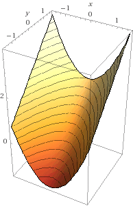
First step. Assume F = ∇f for some potential function f. Gradient Theorem: The line integral of the rate of increase of f along a curve is the total increase along the curve: ∮ ∇f(c) • dc = f(c(1)) − f(c(0)). We can then compute f(a,b) by taking the line integral of ∇f(x,y) from a base point (0,0) to (a,b). This line integral depends only on the endpoints (0,0) and (a,b), and is independent of how c(t) travels between them.
Second step. Suppose F is path indepenent. Given two paths c1, c2 between two points, we can follow the first path out and the second one back to get a closed curve c. Since the line integrals along c1 and c2 are equal, their difference, the line integral around c, is zero. That is, the vector field is irrotational, having zero line integral around any closed curve.
Third step. Curl Theorem: The double integral of the rate of rotation of F over a region R is equal to the total rotation of F around the boundary of R. If F is irrotational, having zero total rotation around any closed curve, this means the rate of rotation at every point must be zero: curl F(x,y) = 0 everywhere.
2d. For F(x,y) = (p(x,y), q(x,y)), the curl F(x,y) = ∂q⁄∂x − ∂p⁄∂y measures how strongly a small paddlewheel at (x,y) would be turned by a fluid flowing with velocity F. A left-to-right increase in the vertical component of F leads to a positive (couterclockwise) curl, hence the term ∂q⁄∂x; a bottom-to-top increase in the horizontal component of F leads to a negative (clockwise) curl, hence the term −∂p⁄∂y.
2e. curl F = ∂⁄∂x(1) − ∂⁄∂y(2x) = 0. Thus F is irrotational, and must have a potential function f.
2f. We compute the potential function f(x,y) at (x,y) = (a,b) as the line integral of F(x,y) = (2x, 1) along the straight-line path c(t) = (at, bt) for 0 ≤ t ≤ 1:
f(a,b) = ∮ F(c) • dc = ∮ F(c(t)) • c'(t) dt = ∮01 F(at, bt) • (at, bt)' dt = ∫01 (2at,1) • (a,b) dt = ∫01 2a2t + b dt = a2 + b.
Thus, f(x,y) = x2 + y, and we can verify that ∇f = F.3a. The quarter-turn ℓ0 takes i to j = (0,1), and j to −i = (−1,0). The corresponding matrix of column-vectors is:
[ ℓ0 ] = 0 −1 1 0 3b. The z-axis quarter-rotation takes i to j, j to −i, and k to itself. These output vectors are the column vectors of the matrix; and similarly for the x-axis quarter-rotation. (Note: we are using the right-handed rotation, in which the thumb points along the positive axis of rotation, and the fingers curl in the rotation direction.)
[ ℓz ] = 0 −1 0 1 0 0 0 0 1 [ ℓx ] = 1 0 0 0 0 −1 0 1 0 3c. Multiplying the above gives the matrix of composite linear mapping ℓz(ℓx(v)):
[ ℓz ∘ ℓx ] = 0 0 1 1 0 0 0 1 0 3d. The columns of the above matrix are the outputs of the coordinate vectors: the mapping takes i → j → k → i. That is, the equilateral triangle with corners at i,j,k is rotated around its center ⅓(i+j+k) = (⅓,⅓,⅓). This means the linear mapping is a 120° rotation around the axis (⅓,⅓,⅓), or equivalently the axis (1,1,1). Note that composing in the other order, ℓx ∘ ℓz, gives a 120° rotation around a different axis.
4a. The Jacobian at (x,y) = (½, 0) of:
f(x,y) = ( (x2+y2)1/2, ((x−1)2+y2)1/2, (x2+(y−1)2)1/2 )
is:[ Df(½, 0) ] = x⁄(x2+y2)1/2 y⁄(x2+y2)1/2 (x−1)⁄((x−1)2+y2)1/2 y⁄((x−1)2+y2)1/2 x⁄(x2+(y−1)2)1/2 (y−1)⁄(x2+(y−1)2)1/2 = 1 0 −1 0 1⁄√3 −2⁄√3 4b. The point (x,y) = (½, 0) is on the line between 0 and i. We can predict the first column of the Jacobian by seeing that moving along the x-axis will have exactly opposite effects on the distances to 0 and i, which accounts for the +1 and −1; while it increases the distance to j at a positive rate, accounting for the bottom entry. As for the second column, moving vertically will affect the distances to 0 and i only tangentially (quadratically), so the first two rows are zero; while the last row is negative, since the vertical motion decreases the distance to j.
4c. The derivative of g(x,y,z) = x+y+z is the row-vector gradient: ∇g(x,y,z) = [1 1 1]. Multiplying a 1×3 matrix by a 3×2 matrix gives a 1×2 matrix, whch is the gradient of g(f(x,y)).
⊞ Problems II: Parametrization, max/min, divergence and flux⊞ Solutions.-
These problems refer to the solid region R inside the
tilted cone
(x−z)2 + y2 ≤ z2, above z = 0, and below the plane
z = 2 − ½x.
- Parametrize R by "conical coordinates".
- Start by parametrizing the top ellipse using polar coordinates with respect to its major and minor axis vectors (from the center to the extreme points), then scale each point (x,y,z) on the ellipse by a parameter s, getting (sx, sy, sz) for 0 ≤ s ≤ 1.
- Use the above parametrization to compute the volume and surface area of R. (Add the areas of ellipse and cone.)
-
Let f(x,y,z) = (x-1)2 + y2 + z2, the square distance of (x,y,z) from (1,0,0).
- From the picture, estimate the critical points of f on R, its boundary surfaces, and its corner boundary circle.
- Find the critical points by solving ∇f(v) = 0 for v ∈ R.
- Find the critical points on the cone and disk surfaces of R by parametrizing them.
- Find the critical points on the corner edge circle (where the surfaces join) by parametrizing it as c(t) and solving f(c(t))' = 0. Also consider the vertex point of the cone.
- Determine the max and min points and values of f on R.
- For the above f, let F = ∇f.
- Sketch this vector field.
- Find div F and curl F, and explain why the answers are expected.
- Determine the integral of div F over R.
- Determine the flux of F through the boundary surfaces of R. Explain why the result is the same as the previous integral.
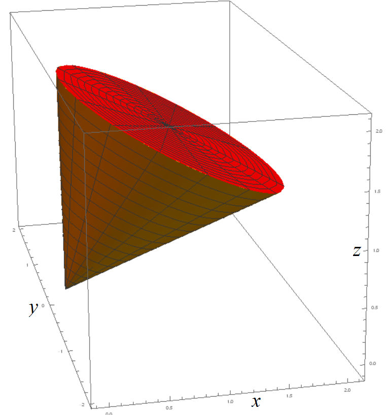 1a. The axis vectors of the ellipse are:
a = (4⁄3,4⁄3,4⁄3) − (4⁄3,0,4⁄3) = (0,4⁄3,0), b = (2,0,0) − (4⁄3,0,4⁄3) = (2⁄3,0,−4⁄3). Then:P(r,t,s) = s ( (4⁄3,0,4⁄3) + r cos(t) a + r sin(t) b ) = (4⁄3 s + 2⁄3 s r sin(t), 4⁄3 s r cos(t), 4⁄3 − 2⁄3 s r sin(t)).
- 12/11 Final Exam: Wed Dec 11, 7:45-9:45am in our usual classroom Wells A-224.
- Weekly Homework to hand in.
-
⊞
WHW 1 due 8/30: Thales' Theorem.
Thales' Theorem in geometry states that if you inscribe a triangle in a half-circle, with one side of the triangle equal to the diameter of the circle, then the angle opposite that side is a right angle. Prove this by vector algebra.
- Here is a model proof for HW 1 #3 above.
- State the proposition to be proved, clearly formulating the hypothesis (the setup or "if" part which is assumed), and the conclusion (the payoff or "then" part to be deduced).
- Start the proof by translating the geometric terms in the hypothesis into vector language. Taking the center of the circle to be the origin, consider the three vertices as endpoints of vectors. Determine the vectors along the relevant sides of the triangle from the vertex opposite the diameter. There is no need to use coordinates: the proof is much cleaner if you keep vectors as letters, not (x,y).
- Use the dot product to test whether the conclusion is true. Carefully expand using the known properties of the dot product, such as commutativity and the distributive law.
- Finally, translate the algebraic conclusion back into geometric language to clinch the conclusion.
- While constructing the proof, you may work forwards from the hypothesis and backwards from the conclusion, hoping to meet in the middle. But in the final draft, you must work only forwards, making each deduction clear.
- You may include a suggestive drawing, but your argument should be readable without it.
- You may turn in hand-written papers, but the best tool to present mathematics is TeX, which you can download free.
- WHW 2 due 9/9: Plane linear mappings, matrix multiplication, rotation & reflection matrices.
-
⊞
WHW 3 due 9/13: Graph landscape.
Invent a function f : R2 → R whose graph z = f(x,y) makes an interesting landscape.
- To start exploring, graph the one-variable bump functions g(r) = 1⁄(1+r2) , 1⁄(1+|r|) , e−r2 (WolframAlpha: plot e^(-r^2) for r=-2.5 to 2.5). Turn each of these curves into a 3D mountain by taking its surface of revolution around the z-axis, namely the graph of the two-variable function f(x,y) = g(√(x2+y2)) (WolframAlpha: plot3d 1/(1+sqrt(x^2+y^2)) for x = -2 to 2 and y = -2 to 2). You can also make a polar coordinate plot, such as z = x2 + y2 over the unit circle. Experiment with other g(r).
- Be artistic. More techniques:
- A long ridge with a given cross-section: z = g(x) or g(y). What is going on with: f(x,y) = exp(−(y−sin(x))2)?
- Experiment with the effect of taking f(x−a, y−b) and f(ax, bx) for some constants a,b.
- Superimpose several mountains and valleys by adding and subtracting such functions.
- Try multiplying functions: exp(−x2−y2) ∗ sin(x) scales the waves of f(x,y) = sin(x) by the bump function exp(−x2−y2).
- Taking the square root of a positive function produces cusps at the zero points: egg-crate function f(x,y) = −√(2−cos(x)−cos(y)).
- Functions of the form f(x,y) = g(x) + h(y) can be visualized by drawing the backbone z = g(x) above the x-axis, then hanging perpendiuclar copies of z = h(y) along the backbone, with the copy above a given line x = c being raised by g(c).
- Find the (x,y) window which best shows the
interesting features of your function.
In addition to the graph, take the contour plot and gradient vector field.
Hint: It is probably best to draw the gradient vectors by hand onto the contour plot: remember that the closer the contours, the longer the gradient (since its length is the uphill slope). - Once you have your function, locate its critical points, which are the flat points on its graph. These are the values (x,y) where ∇f(x,y) = (df⁄dx,df⁄dy) = (0,0). (W|A will solve the equations for you most of the time.) Classify each as a min (valley like z = x2+y2), max (hill like −x2−y2) or saddle (like x2−y2), or possibly a ditch or ridge (like ±x2). Note how each of these looks on the countour plot and gradient field.
- Software tips.
- WolframAlpha functions: plot curves, surfaces, polar plot surfaces vector fields; multiply matrices.
- You might want to pay $5 for a month of Wolfram|Alpha Pro, which makes W|A work a good deal better (for example, it accepts long inputs).
- A more powerful option is Wolfram Mathematica, free from MSU.
Turn in:
- For your most interesting-looking function f(x,y), a printout of the graph, countour plot and gradient vector field (copy and paste the W|A images).
- A clear description of how you built up the formula for your function f(x,y) from its basic elements. Explain how each part of the formula controls some feature of the picture, not just "I tried this formula at random, and the computer drew that picture, I don't know why."
- Location and classification of the critical points. (At least give approximate location if solving the equations is too difficult.)
- WHW 4 due 9/20: Optimizing a sawmill.
- WHW 5 due 9/30: Parametrization mappings, affine approximation, Jacobian matrix.
- WHW 6 due 10/7: Mean Value Theorem and two definitions of curl.
- WHW 7 due 10/14: Computing double integrals.
-
⊞
WHW 8 due 10/21: Conservative Vector Field Theorem.
All of the following conditions are equivalent for a vector field F(x,y):
- F is conservative: there is a potential function f with F = ∇f.
- F is path independent: the line integral between two fixed points is the same for any choice of path between them: for any paths c1, c2 with c1(0) = c2(0) = (a,b) and c1(1) = c2(1) = (c,d), we have ∫ F(c1)•dc1 = ∫ F(c2)•dc2 .
- F has zero circulation: the line integral around any loop is zero: if c(t) for 0 ≤ t ≤ 1 is a closed curve with c(0) = c(1), then ∮ F(c)•dc = 0.
- F is irrotational: curl F(x,y) = 0 at all (x,y).
Hints: Model (latex)- We previously discussed the Conservative Vector Field Theorem in Lect 15.
- As in all proofs, start by stating the Theorem at the beginning, briefly: you don't need to include definitions of your terms.
- In each section of the proof, start by stating the hypothesis (the setup assumed) and end by stating the conclusion deduced.
- You may use any theorems we have covered, explicitly referenced to the Lecture number above where they appear. (Looking these up is a good way to review.)
- (i) ⇒ (ii): Use the Gradient Theorem ∫ ∇f(c)•dc = f(c(1)) − f(c(0)).
- (ii) ⇒ (iii): For a curve c(t) with
0 ≤ t ≤ 1, and its reverse curve
c−(t) = c(1−t),
show that ∫ F(c−)•dc−
= −∫ F(c)•dc
using the single-variable Substitution Theorem:
for u = g(t) = 1−t, we have:
∫ab f(g(t)) g'(t) dt = ∫g(a)g(b) f(u) du. Then, for a given loop, cut it into two paths from the beginning point to the half-way point. - (iii) ⇒ (iv): Use the limit definiton of curl from WHW 6:curl F(x,y) = limc→(x,y) ∫ F(c)•dc⁄area(c) .
- (iv) ⇒ (iii): Use the Curl Theorem
∬D curl F(x,y) dx dy
=
∮ F(c)•dc,
where c is the counterclockwise boundary of a region D.
Note: This proves (iii) only for curves which bound a region D, but you may ignore more complicated curves (such as self-intersecting ones). - (iii) ⇒ (ii): Easy converse of (ii) ⇒ (iii).
- (ii) ⇒ (i): Here you need a real argument.
Assume that the line integral of F = (p,q) from (0,0) to (x,y)
is a function f(x,y) depending only on (x,y), not on the path chosen;
then you must show ∂f⁄∂x = p
and ∂f⁄∂y = q.
For the first, compute f(x,y) along the rectangular path from (0,0) to (0,y) to (x,y), and use the single-variable First Fundamental Theorem of Calculus, applied to the variable x as a bound of integration. That is, if you parametrize the path correctly, f(x,y) = ∫0x p(t,y) dt + (term without x), and ∂f⁄∂x(x,y) = p(x,y), as desired. So far, this will work for any F. But now, assuming path independence, you get the same f(x,y) from the other rectangular path, and show the other formula ∂f⁄∂y = q(x,y).
- Extra Credit HW due Thu 10/31: Thickened curves. (tex, Mathematica)
-
⊞
WHW 9 due 11/7: Parametrized curves and surfaces in space.
Solutions (Mathematica).
For each surface:
- Write a parametric formula
P(t,s) = (x(t,s), y(t,s), z(t,s))
over a parameter region S* in the (t,s)-plane.
Use whatever parameter variables you like: P(θ,φ), etc. - Print out a picture of the surface. (Plotting software: W|A, Mathematica (Example), Zweig, Desmos, URI.)
- Helix curve (corkscrew, spring) coiling upward around the z-axis and above the xy unit circle (radius 1)
- Helical staircase surface, consisting of horizontal rays from z-axis to helix
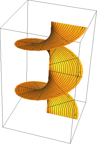
- Tube surface at distance r from the helix. Hint: Use the Frenet frame from Lect 27.

- Ram's horn
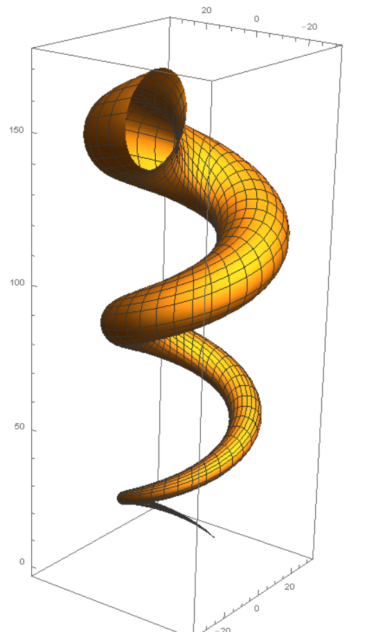
- Elliptical surface on a tilted plane, with major axis
from a = (1,2,3) to −a = (−1,−2,−3), and minor axis from
b = (2,−1,0) to −b = (−2,1,0). Note a ⊥ b.
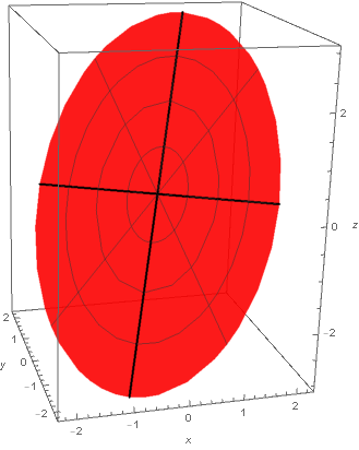
- Spherical coordinates on the globe
- Draw a globe surface with some mountains on it,
adapting some of the topographic features from WHW 3.
In that project, we regarded the globe from up close,
treating longitude, latitude, altitude as rectangular coordinates.
Now use Sph to transfer those pictures to a sphere.
- Draw line segments between the following
consecutive (latitude, longitude) points,
making a polygon:
(-124, 49), (-90, 49), (-83, 42), (-70, 47), (-67, 45), (-82, 31), (-81, 25), (-84, 31), (-94, 31), (-98, 26), (-108, 32), (-117, 32), (-124, 40), (-124, 49) Mathematica: Graphics[Polygon[{{x1,y1}, {x2,y2}, . . . }]]; or try GeoGebra: calculator icon, command Polygon((x1,y1), (x2,y2), . . .), click Settings icon, Zoom to fit.
What does this represent? Why does it look too wide?
Extra Credit: Use the appropriate linear mapping to convert (latitude, longitude) into (θ,φ), and use Sph(4000, θ, φ) to draw the corresponding polygon on the globe (radius 4000 mi). - On a map, find a latitude-longitude rectangle D* that roughly approximates the map of the continental United States. For the corresponding region D = Sph(D*) on the Earth, compute its area using the area substitution formula. That is, fixing the Earth's radius at ρ = 4000 mi, parametrize the globe as P(θ,φ) = Sph(4000,θ,φ) and compute: Area = ∫∫D* |∂P⁄∂θ×∂P⁄∂φ| dθ dφ . How well does this match the actual area of the continental U.S.?
- Draw a globe surface with some mountains on it,
adapting some of the topographic features from WHW 3.
In that project, we regarded the globe from up close,
treating longitude, latitude, altitude as rectangular coordinates.
Now use Sph to transfer those pictures to a sphere.
- Write a parametric formula
P(t,s) = (x(t,s), y(t,s), z(t,s))
over a parameter region S* in the (t,s)-plane.
- WHW 10 due Thu 11/14: Limits and error analysis. (tex)
- WHW 11 due Wed 12/11: Final review problems. (tex)
- Notes & Tools
- Review notes on Calculus I and Calculus II.
- Marsden & Tromba Theoretical Supplement
- Calculus explainer: 3BLUE1BROWN
-
⊞
Software
- Wolfram Alpha plotting
- parametric curve c(t) = (x(t), y(t))
- contour plot f(x,y) = c
- graph surface z = f(x,y)
- polar plot z = x2 + y2 over unit circle
- vector field F(x,y) = (p(x,y), q(x,y))
- 3D parametric surface F(u,v) = (x(u,v), y(u,v), z(u,v))
- multiply matrices
- Get Wolfram Mathematica with a free MSU license. Plotting: 2D, 3D.
- Surface plotters: GeoGebra, Zweig, Desmos, URI
- Wolfram Alpha plotting
Old Math 254H: Spring 2016, Spring 2017
- With colored pens, plot straight grid lines in the (r,θ) plane corresponding to r = 0, 1, 2, 3, and θ = 0, π⁄4, π⁄2, 3π⁄4, . . . , 7π⁄4, and the corresponding grid curves
in the (x,y) plane, under the polar mapping
- Function F : R2 → R2,
F(u,v) = (f1(u,v), f2(u,v)) = (x(u,v), y(u,v))