8.  Orthogonality and Least Squares

§8.1 Orthogonality

    We start with vector orthogonality.  Two vectors x and y  are said to be orthogonal if their inner product is 0; i.e., < x, y > =  x^T*y = 0.  Remember that the MATLAB command that calculates inner products looks like

>> x'*y

    Enter the following vectors into MATLAB.  Remember to use semicolons between entries so that you produce column vectors.

Exercise 8.1
	(a)  Check the above five vectors for orthogonality.  List all possible combinations of orthogonal sets.
	(b)  Pick a maximum set from part (a) that is linearly independent and normalize all the vectors using the following command: >> v = (1/norm(v))*v The above will normalize the vector v. That is, we use the norm() command to calculate the norm of the vector v and then we divide by the norm to get a vector of length 1. Now, explain why can't there be more than four orthogonal vectors in the above set?

For the next exercise we are going to use the following three vectors

Remark 8.1 The above vectors are orthonormal. Hence we can create an orthogonal matrix.

Enter the above vecotrs into MATLAB. Use the following command to create an orthogonal matrix Q

>> Q = [f g h]

Exercise 8.2
	(a)  Calculate QT*Q.  What do you get?  Why should we expect this result?
	(b)  Enter the following vectors into MATLAB: Compute the norm of b and the norm of Q*b.  What do you notice?  Compute aT*b and compare it to (Q*a)T*(Q*b).
	(e)  It should be clear that our matrix Q is invertible (the columns are linearly independent as the vectors are othogonal.)  Hence we can compute Q-1.  Use inv(Q)to compute the inverse of Q and compare it to QT.  Is what you notice a surprise to you?  Explain.

§8.2 Orthogonal Projections and Gram-Schmidt Process

    First, we will look at orthogonal projections onto a vector.  Hopefully, you were able to determine in §8.1 above that the vectors v and x are not orthogonal.  (Projections are trivial if the vectors are orthogonal, all one has to do is choose 0 as the orthogonal projection.)  Suppose we want to find the orthogonal projection of v onto x, let's denote it by v.  Then the formula tells us that

v = (v^T*x)/(x^T*x)*x

Here's a pictorial depiction of what we are doing

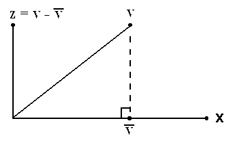
Remark 8.1 It is not possible to enter v into MATLAB. Instead, when defining the vector v call it vbar.

Exercise 8.3
	(a)  Find v = (the orthogonal projection of v onto x) and z = (the component of v orthogonal to x.) Then write v as the sum of these two vectors.
	(b)  Show that z is orthogonal to v.

    The idea of projecting a vector onto a subspace is easily extended from the above case by looking at an orthogonal basis for the subspace, projecting the vector onto each basis element, and then adding them all up to form the orthogonal projection.

    All this brings us to the Gram-Schmidt process.  Fortunately for us, MATLAB can do the QR Factorization right away using the qr() command.

Example 8.1 

    Let's try to find an orthonormal basis for the subspace spanned by our two vectors a and b. We start by defining a new matrix A with a and b as its columns.

>> A = [a b]

    A =

            1     2
            1     0
            0     3

Next, we apply the qr() command.

>> [Q,R]=qr(A)

    Q =

        -0.7071     0.3015    -0.6396
        -0.7071    -0.3015     0.6396
         0          0.9045     0.4264


    R =

        -1.4142     -1.4142
         0           3.3166
         0           0

Remark 8.1  There is a slight ambiguity above that results from the fact that our matrix is not square. The output consists of a 3x3 matrix Q. But when we perform Gram-Schmidt on our two vectors we should get two (instead of 3) orthonormal vectors. That is why we are going to use a shortened version of the command. Type the following and notice the difference in output

>> [Q,R]=qr(A,0)

    Q =

        -0.7071     0.3015
        -0.7071    -0.3015
         0          0.9045


    R =

        -1.4142     -1.4142
         0           3.3166

    We get that the orthonormal basis for the subspace spanned by a and b is

Exercise 8.4  The following is a basis for R3: Turn it into an orthonormal basis. Check that, in fact, the basis is orthonormal.  (Check for orthogonality and look at the norms.)

§8.3 Least Squares

    Suppose we are interested in studying the relationship between temperature and pressure.  The first step is to obtain some experimental data.  In order to do that, we attach a temperature and pressure sensor to a metal container.  Starting at the room temperature (75°F) we slowly heat the air inside our container to 195°F and record temperature and pressure readings.  We get a total of five data points

    Since we suspect the relationship to be linear, we will be looking for a straight line with the following equation y = mx +b, where y is the pressure, x the temperature, m the slope, and b the y-intercept.

    Our goal becomes to solve the following system of linear equations:

    Unfortunately, the system does not have a solution, even though the physical law is of linear order. This is due to the fact that it is not possible to get perfect accuracy when recording data.  Our instruments are limited, and there is always the human error.

    Since it is not possible to solve the above system, we use the least squares method to find the closest solution.  That is, we want to get the best fit line.

Remark 8.2  By best fit line we mean a line that minimizes the sum of the squares of the distances from each point to the line.

To simplify notation let's assign letters to the matrices and vectors of the above system. 

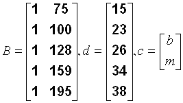
We can find our best-fit coordinates by solving B^T*B*c=B^T*d, i.e. c=(B^T*B)^-1*B^T*d.  (This only works because B^T*B is nonsingular.)

 

	Exercise 8.5
	(a)  Use MATLAB to compute c.
	(b)  What is the equation of our line?
	(c)  We can now plot the data points and our line to see visually if the approximation is good or not.  Type the following: >> x=B(:,2); >> y=d; >> t=0:1:300; >> z=polyval([c(2);c(1)],t); >> plot(x,y,'x',t,z)
	(d)  Calculate the pressure at the following temperatures 70°F, 125°F, and 225°F.

Remark 8.3  polyval()returns a polynomial of specific degree with coefficient specified by a vector.

§8.4 Conclusion

    Least squares are quite useful in analyzing all sorts of experimental data. As long as we have some idea about the relationship between the data, we can use least squares to make predictions and extend the results beyond the scope of our experiment.

Last Modified:

03/26/2005