My research interest focuses on the Schramm-Loewner evolution (SLE for short), which describes some random fractal curves in plane domains whose distribution is preserved under conformal (analytic and one-to-one) maps. It was introduced by Oded Schramm in 1999 to study the scaling limits of loop-erased random walk in the plane. The definition combines the Charles Loewner’s equation (1923) from Complex Analysis with a random input function. Loewner’s equation generates a map from C([0,T],R) to the set of “curves” in plane domains. If the input function is times a standard Brownian motion then the random curve obtained is called SLE with parameter κ; and we write SLE_κ to emphasize this parameter.

The merit of SLE is that one can now use the tools from Stochastic Analysis to analyze some random curves in the plane. Such curves include the scaling limits of many two dimensional statistical physics models, e.g., critical site percolation, Ising models at critical temperature, Gaussian free field, loop-erased random walk, and uniform spanning tree. These lattice models have been proved to converge to SLE with different parameters. Another important application of SLE is that it was used to prove Mandelbrot’s conjecture: the boundary of plane Brownian motion has fractal dimension 4/3.

Of many variants of SLE, the chordal SLE and radial SLE are most well-known. They are both defined in simply connected domains. A chordal SLE curve grows from one boundary point to another boundary point; a radial SLE curve grows from a boundary point to an interior point.

One of my research projects is to extend SLE to multiply connected domains, and relate them to lattice models in these domains. I have defined SLE in doubly connected domains by introducing a new kind of Loewner equation. Latter I defined a family of SLE in multiply connected domains using the traditional Loewner’s equation, and proved that they are the scaling limits of loop-erased random walk in these domains. One may consider the scaling limits of other lattice models in multiply connected domains.

My recent interest is the application of a new tool in the area of SLE: the stochastic coupling technique. Roughly speaking, the coupling technique allows two SLE curves to grow in the same plane domain simultaneously. If these two curves satisfy that every point on one curve will be visited by the other, then they overlap. The first application of this technique was to show that chordal SLE_κ satisfies reversibility if κ≤4. This means that the chordal SLE_κ curve from a to b is the same as the chordal SLE_κ curve from b to a. This technique was also used to show the duality of SLE: the outer boundary of an SLE_κ curve with κ>4, which is not a simple curve, has the shape of an SLE_16/κ curve. Here the parameter 16/κ is the dual of κ. It is known that SLE_κ and SLE_16/κ have the same central charge. The coupling technique may also be used to study the reversal curve of radial SLE. Another interesting application is that one may erase loops on a plane Brownian motion in the order they appear to get a simple curve, which is an SLE₂ curve.

Here are a few pictures from the area of SLE.
Figure 1: The red part is a plane Brownian motion in the disc (approximated by random walk on a square lattice with very small mesh). The black curve is the outer boundary of this Brownian motion. The boundary curve has fractal dimension 4/3, which was conjectured by Mandelbrot, and proved by G.F. Lawler, O. Schramm, and W. Werner using SLE. In fact, it is an SLE_8/3 curve.

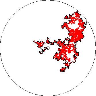
Figure 2: The hexagon faces on the bottom lines are colored in such a way that the left half of them are colored gray, and the right half of them are colored white. All other hexagons are colored gray or white independently with probability 1/2. The red line runs along the boundaries of the hexagons in such a way that the hexagons on its left is gray, and the hexagons on its right is white. When the size of the hexagons tends to 0, this red curve converges to SLE₆ (by S. Smirnov).

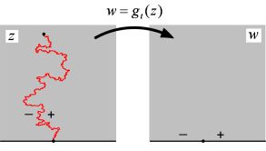
Figure 3: This zigzag curve on the left is an SLE curve. The function g_t is a conformal map that maps the upper half plane without the curve (up to time t) onto the whole upper half plane. The curve is understood as a part of the boundary of the domain, and g_t maps the two sides of the curve onto two real intervals. The variable t is the time parameter of the curve. The family of maps {g_t} satisfies Loewner's equation. The way that SLE people analyze the fractal curve is to study the functions {g_t} instead.